Decode any math function in minutes: A Step-by-Step Framework powered by AI

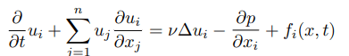
Example Navier-Stokes equation:

Show an example of the output or outcome of this function?

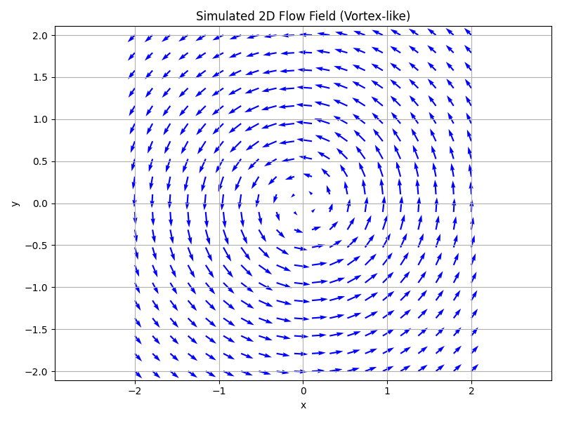
Example: 2D Vortex Flow

Let’s consider a simple 2D example: a decaying vortex in a viscous fluid. This is a classic solution to the Navier-Stokes equations in two dimensions.

Setup:

• No external force: ( f_i(x, t) = 0 )
• Initial velocity field: circular vortex
• Viscosity ( \nu > 0 )

Outcome:

Over time, the vortex slows down and diffuses due to viscosity. The velocity field becomes smoother, and the rotational motion weakens.

What exactly is this function trying to teach? What problem does this help me solve?

What is it trying to teach?

It models how fluids (like air, water, oil, etc.) move and behave under various conditions. Specifically, it teaches:

• Momentum conservation in a fluid.
• How velocity, pressure, viscosity, and external forces interact.
• The balance between inertia, pressure gradients, viscous diffusion, and external forces.

What problems does it help solve?

The Navier-Stokes equations are used to solve real-world problems involving fluid flow. Here are some examples:

1. Engineering & Design

• Aerodynamics: Designing cars, airplanes, and drones for optimal airflow.
• Hydraulics: Modeling water flow in pipes, dams, and irrigation systems.

2. Weather & Climate

• Predicting weather patterns, storms, and climate dynamics.

3. Medicine & Biology

• Simulating blood flow in arteries or airflow in lungs.

4. Environmental Science

• Modeling pollution dispersion in air or water.
• Understanding ocean currents and atmospheric circulation.

5. Computer Graphics & Animation

• Creating realistic fluid simulations in movies and video games.

Why is it challenging?

Despite its importance, solving the Navier-Stokes equations analytically is extremely difficult in most cases. That’s why we often use numerical simulations (like Computational Fluid Dynamics, CFD) to approximate solutions.

Instead of using mathematical symbols, express the function entirely in words.

The rate of change of the fluid’s velocity in a given direction, plus the combined effect of all the fluid’s velocity components interacting with each other across space, is equal to the influence of viscosity spreading the velocity out, minus the change in pressure in that direction, plus any external force acting on the fluid at that location and time.

Breaking it down further:

1. Rate of change of velocity: How fast the fluid’s speed is changing over time in a specific direction.
2. Advection (nonlinear interaction): How the fluid’s own movement affects its velocity—like how a current carries itself forward.
3. Viscous diffusion: The smoothing effect of internal friction (viscosity), which spreads out sharp changes in velocity.
4. Pressure gradient: How differences in pressure push the fluid from high-pressure areas to low-pressure areas.
5. External forces: Any outside influence like gravity, magnetic fields, or applied forces that affect the fluid’s motion.

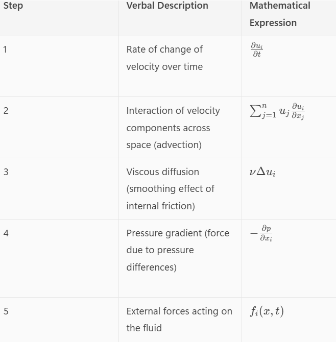
Now, list the descriptions in words (steps 1 to 5) in a table, and show how each one relates to the corresponding mathematical expression in the function.

Step	Verbal Description	Mathematical Expression	Meaning
1	Rate of change of velocity over time	\frac{\partial u_i}{\partial t}	How fast the fluid’s velocity is changing at a point in time.
2	Interaction of velocity components across space (advection)	\sum_{j=1}^n u_j \frac{\partial u_i}{\partial x_j}	How the fluid’s own motion carries and changes its velocity.
3	Viscous diffusion (smoothing effect of internal friction)	\nu \Delta u_i	How viscosity spreads out sharp changes in velocity.
4	Pressure gradient (force due to pressure differences)	-\frac{\partial p}{\partial x_i}	How pressure differences push the fluid in a certain direction.
5	External forces acting on the fluid	f_i(x, t)	Any outside influence like gravity, magnetic fields, or applied forces.

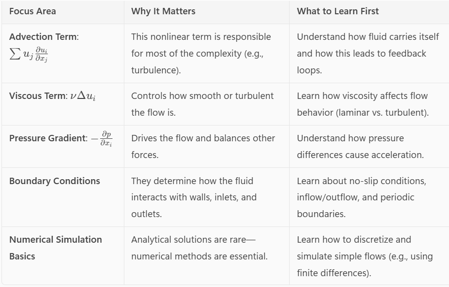
Which parts are worth focusing on first (80/20)?

Apply all these frameworks to above mathematical function

1. Structural Analysis Domain & Codomain:
What inputs are allowed?
What outputs are possible?
Continuity & Differentiability: Is the function smooth?
Are there jumps or corners?
Symmetry: Even, odd, periodic?
Monotonicity: Increasing, decreasing, or constant?
2. Graphical Interpretation Plot the function:
Visualizing the function often reveals behavior (e.g., asymptotes, extrema, inflection points). L
evel sets / Contour plots (for multivariable functions): Show where the function takes constant values.
3. Algebraic Tools Taylor Series / Approximations:
Understand local behavior near a point.
Factorization / Simplification: Reduce complexity to reveal structure.
Limits and asymptotics: Understand behavior at boundaries or infinity.
4. Functional Perspective Linear vs. Nonlinear:
Linear functions are easier to analyze and often serve as approximations. Convexity: Important in optimization—convex functions have global minima. Operator View: In functional analysis, functions can be seen as operators acting on spaces.
5. Computational Tools Symbolic computation (e.g., WolframAlpha, SymPy): For derivatives, integrals, simplifications.
Numerical evaluation: Plug in values to get a feel for the function.
Automatic plotting: Tools like Desmos, GeoGebra, or Python (Matplotlib, Plotly).
6. Contextual Frameworks Optimization:
Is the function a cost, utility, or energy function?
Control theory: Is it part of a system dynamic?
Physics / Engineering: Does it model a real-world phenomenon?
7. Heuristic Questions Ask yourself:
What happens as x→∞ x→∞ or x→0 x→0?
Where is the function zero?
Where is it undefined?
What are the critical points?

🔍 1. Structural Analysis

Aspect	Explanation
Domain	Space (x, y, z) and time (t)
Codomain	Vector field (velocity components in 3D)
Continuity	Assumes smooth, differentiable velocity and pressure fields
Symmetry	No inherent symmetry unless imposed by boundary conditions
Monotonicity	Not monotonic; fluid behavior is dynamic and can oscillate or reverse direction

📈 2. Graphical Interpretation

• Plotting: Direct visualization is complex due to the vector and PDE nature, but simulations show vortices, turbulence, and laminar flow.
• Level Sets / Contours: Often used to visualize pressure or velocity magnitude in 2D slices of the domain.

🧮 3. Algebraic Tools

Tool	Insight
Taylor Series	Used to linearize the equation near steady states (e.g., for stability analysis)
Simplification	In low Reynolds number (viscous-dominated), convective terms can be neglected
Limits & Asymptotics	At high Reynolds numbers, turbulence and chaotic behavior emerge

🧠 4. Functional Perspective

Aspect	Classification
Linearity	Nonlinear, due to the convective term ( (u \cdot \nabla)u )
Convexity	Not convex; multiple solutions and instabilities are possible
Operator View	A differential operator acting on velocity and pressure fields

🧰 5. Computational Tools

• Symbolic Tools: Used to derive and manipulate the equations (e.g., SymPy, Mathematica)
• Numerical Solvers: Finite element, finite volume, and spectral methods (e.g., OpenFOAM, ANSYS Fluent)
• Visualization: Matplotlib, ParaView, or CFD software for flow field visualization

🧭 6. Contextual Frameworks

Field	Application
Optimization	Used in flow control problems (e.g., minimizing drag)
Control Theory	Applied in feedback control of fluid systems (e.g., HVAC, drones)
Physics/Engineering	Core to fluid dynamics, aerodynamics, weather modeling, and biomedical flows

🧠 7. Heuristic Questions

Question	Answer
What happens as ( x \to \infty )?	Depends on boundary conditions; often assumed to decay to zero
Where is the function zero?	When velocity and external forces are zero
Where is it undefined?	Singularities may occur in turbulent or chaotic flows
What are the critical points?	Where velocity gradients vanish or change sign (e.g., stagnation points)

Who gave the best-ever explanation of this function so that even people with no mathematical background could understand it, and how did they explain it?

🧠 Who explained it best?

Dr. Steven Strogatz

• Professor at Cornell University
• Contributor to The New York Times and author of popular science books like The Joy of x

---

📖 How did he explain it?

In his writing and talks, Strogatz breaks down the Navier-Stokes equations using everyday analogies and plain language. Here’s a simplified version of his approach:

---

🌀 1. Think of Fluid as a Crowd of Tiny Particles

He invites readers to imagine a fluid as a swarm of tiny particles—like a crowd of people moving through a city.

🧭 2. What Influences Their Motion?

Each particle’s motion is influenced by:

• Inertia: It wants to keep moving in the same direction.
• Pressure: Like people moving away from a crowded area.
• Viscosity: Like friction between people slowing each other down.
• External forces: Like wind or gravity pushing the crowd.

🧮 3. The Equation is a Balance Sheet

He describes the Navier-Stokes equation as a balance sheet:

• On the left: how the velocity of the fluid is changing.
• On the right: all the reasons why it’s changing (pressure, viscosity, forces).

🎨 4. He Uses Visual Metaphors

Instead of diving into symbols, he uses visual metaphors:

• Flowing honey vs. rushing water
• Smoke swirling in air
• Traffic jams as analogies for pressure buildup

🧩 Why it works so well:

• No equations at first—just intuition.
• Relatable metaphors—like crowds, traffic, and weather.
• Builds curiosity—then introduces the math once the concept is clear.

---

Frameworks for Understanding Mathematical Functions

🔍 1. Structural Analysis

• Domain & Codomain: What inputs are allowed? What outputs are possible?
• Continuity & Differentiability: Is the function smooth? Are there jumps or corners?
• Symmetry: Even, odd, periodic?
• Monotonicity: Increasing, decreasing, or constant?

📈 2. Graphical Interpretation

• Plot the function: Visualizing the function often reveals behavior (e.g., asymptotes, extrema, inflection points).
• Level sets / Contour plots (for multivariable functions): Show where the function takes constant values.

🧮 3. Algebraic Tools

• Taylor Series / Approximations: Understand local behavior near a point.
• Factorization / Simplification: Reduce complexity to reveal structure.
• Limits and asymptotics: Understand behavior at boundaries or infinity.

🧠 4. Functional Perspective

• Linear vs. Nonlinear: Linear functions are easier to analyze and often serve as approximations.
• Convexity: Important in optimization—convex functions have global minima.
• Operator View: In functional analysis, functions can be seen as operators acting on spaces.

🧰 5. Computational Tools

• Symbolic computation (e.g., WolframAlpha, SymPy): For derivatives, integrals, simplifications.
• Numerical evaluation: Plug in values to get a feel for the function.
• Automatic plotting: Tools like Desmos, GeoGebra, or Python (Matplotlib, Plotly).

🧭 6. Contextual Frameworks

• Optimization: Is the function a cost, utility, or energy function?
• Control theory: Is it part of a system dynamic?
• Physics / Engineering: Does it model a real-world phenomenon?

🧑‍🏫 7. Heuristic Questions

Ask yourself:

• What happens as ( x \to \infty ) or ( x \to 0 )?
• Where is the function zero?
• Where is it undefined?
• What are the critical points?