The NAND Gate of Continuous Mathematics: A Review of the EML Operator and its Interdisciplinary Implications (eg IMAP MISSION, SpaceWeather Forecasting)

Abstract

In Boolean logic, functionally complete primitive gates (like NAND or NOR) form the foundational basis of all digital computation. Historically, continuous mathematics lacked an equivalent unifying primitive, instead relying on a disjointed vocabulary of distinct elementary functions (addition, multiplication, trigonometry, logarithms). In April 2026, Andrzej Odrzywołek introduced the Exp-Minus-Log (EML) operator, demonstrating that a single binary operator, when combined with the constant 1, is sufficient to generate the entire standard repertoire of a scientific calculator [1]. This review synthesizes the foundational theory of the eml operator, its transformative potential in gradient-based symbolic regression, its emerging open-source software ecosystem, and the critical debates surrounding its physical implementation in hardware architectures.

Based on this review, the eml operator will be applied to the data collected by the IMAP (Interstellar Mapping and Acceleration Probe) Mission [7]. The focus is in the first step on solar wind turbulence utilizing plasma [8] and magnetic field [9] telemetry, and in the second step on the energetic particle mapping.

Palme, P. (2026). Autonomous Recovery of Chaotic Plasma Couplings: An EML-Based Neural ODE Framework for the IMAP Mission. Zenodo. https://doi.org/10.5281/zenodo.20169007

1. Theoretical Foundations: Functional Completeness in Continuous Mathematics

In his foundational preprint, All elementary functions from a single binary operator, Odrzywołek proves that the continuous operator defined as:

eml(x,y) = exp(x) – ln(y)

acts as a universal primitive for continuous mathematics. Discovered via a systematic computational ablation search over 36 standard mathematical primitives, the operator allows for the construction of all fundamental algebraic and transcendental functions.

Because the operator leverages the complex domain and the principal branch of the logarithm, it acts as a bridge between additive/multiplicative arithmetic and complex circular functions. For example:

Exponentiation: exp(x) = eml(x,1)
Logarithms: ln(x) = eml(1,eml(eml(1,x),1))
Constants: The constant e evaluates to eml(1,1), while deeper recursive compositions yield pi and the imaginary unit i.

The mathematical grammar is exceptionally strict and uniform: S t-> 1 | eml(S, S). Every valid mathematical expression is isomorphic to a full binary tree containing only identical eml nodes and terminal leaves of variables or the constant 1.

2. Impact on Artificial Intelligence and Symbolic Regression

The most immediate and profound application of the eml operator is in the field of artificial intelligence, specifically symbolic regression—the extraction of closed-form physics equations from empirical data.

Traditional symbolic regression struggles with a highly irregular search space; standard operators have different domains, rules, and computational costs. Odrzywołek’s discovery flattens this landscape entirely. Because any elementary formula can be rewritten as a perfectly uniform binary tree of eml nodes, the search space becomes a context-free language.

Researchers can now parameterize these trees and train them using standard continuous optimization techniques (like the Adam optimizer). As the model converges on experimental data, the continuous weights snap to exact binary topologies, allowing black-box neural architectures to output exact, human-readable scientific equations[1].

3. The Software Ecosystem: Compilers and Emulators

The software engineering community’s response to the paper was remarkably swift, leading to the development of early experimental compilers and evaluation tools.

oxieml: A pure Rust crate built to parse, evaluate, and generate eml expressions. It acts as an algorithmic translation layer, converting standard abstract syntax trees (ASTs) into deep eml trees and emitting optimized code. It also explores SMT (Satisfiability Modulo Theories) integration for constraint solving via tree interval narrowing [3] .
emlmath: Another Rust utility operating as a testbed for branch-cut and complex-analysis behavior. It highlights a critical scaling issue: while theoretically elegant, expressions like basic addition (x + y) require five layers of nesting, causing the compiled eml expression trees to grow exponentially large [4].

4. Hardware Engineering and FPGA Implementations

While AI researchers embraced the uniform topology, the hardware engineering community has heavily scrutinized the operator’s physical viability. Direct translation of an eml tree into Register-Transfer Level (RTL) logic on Field Programmable Gate Arrays (FPGAs) is highly inefficient. Computing exp and ln are resource-heavy, multi-cycle operations; physically chaining them consumes exorbitant amounts of DSP slices and Block RAM (BRAM).

However, hardware analysts have identified a highly viable niche: Microcoded Mathematical Processors. Rather than building deeply nested physical trees, engineers propose utilizing a single eml Arithmetic Logic Unit (ALU). By pairing this single ALU with a small (16-32 entry) memory stack, a Program ROM, and a Finite State Machine (FSM), FPGAs can evaluate complex functions by sequencing operations over time. This architecture trades throughput for ultimate flexibility, making it highly attractive for resource-constrained edge computing devices where silicon footprint is more critical than clock speed [5] .

5. Critiques and Mathematical Edge Cases

Despite its elegance, the EML framework faces significant numerical and theoretical hurdles:

Partial Functions and Singularities: Critics have noted the inherent danger of using ln(y) as a foundational building block. Because ln(0) introduces singularities, it is impossible to guarantee that an arbitrary, deep eml tree is well-defined across all inputs. “You cannot generate a total function from a partial function” remains a core theoretical critique.
Floating-Point Error Propagation: In digital architectures, ln(y) relies on polynomial approximations, introducing minor quantization errors. When these errors are fed into the exp(x) portion of subsequent eml nodes, the errors are exponentially amplified, leading to severe floating-point drift in deep trees [6].

Conclusion

Andrzej Odrzywołek’s eml operator represents a paradigm shift in how computer science and continuous mathematics intersect. While its susceptibility to floating-point drift and hardware latency makes it impractical as a direct replacement for traditional floating-point units, its ability to unify the search space of symbolic regression provides a revolutionary new tool for AI-driven scientific discovery. The eml operator proves that the underlying “source code” of continuous mathematics is vastly simpler than centuries of pedagogy previously suggested.

References

[1] A. Odrzywołek, “All elementary functions from a single binary operator,” arXiv preprint arXiv:2603.21852, Mar. 2026. Available: https://arxiv.org/abs/2603.21852.

[2] “emlmath: A scientific math library based on the paper All elementary functions from a single binary operator,” Crates.io, version 0.1.0, Apr. 2026. [Online]. Available: https://crates.io/crates/emlmath.

[3] OxiEML, GitHub Repository, 2026. [Online]. https://github.com/cool-japan/oxieml

[4] emlmath, GitHub Repository, 2026. [Online]. https://lib.rs/crates/emlmath

[5] MicroZed Chronicles: EML in FPGA https://www.adiuvoengineering.com/post/microzed-chronicles-eml-in-fpga#:~:text=Critically%2C%20each%20node%20in%20the,directly%20implementing%20the%20required%20function.

[6] “Comment on ‘All elementary functions from a single binary operator’,” Reddit, r/math, 2026. [Online]. Available: https://www.reddit.com/r/math/comments/1sk63n5/all_elementary_functions_from_a_single_binary/

[7] D. J. McComas et al., “Interstellar Mapping and Acceleration Probe (IMAP): A New Window on the Heliosphere,” Space Science Reviews, vol. 214, no. 8, p. 116, Oct. 2018. doi: 10.1007/s11214-018-0550-1.

[8] C. J. Joyce et al., “The Solar Wind and Pickup Ion (SWAPI) Instrument for the IMAP Mission,” Space Science Reviews, vol. 220, no. 3, 2024. (Note: Crucial citation for the plasma velocity data you are using for the turbulence model).

[9] T. S. Horbury et al., “The IMAP Magnetometer (MAG),” Space Science Reviews, vol. 220, no. 1, 2024. (Note: Crucial citation for the magnetic field data).

Topic	Confidence score
L1 MAG Data Quality for Analysis (0 readings for variables but overall magnetic field magnitude > 0)	80-90%
L1 SWAPI Data Quality for Analysis (No zero readings)	80-90%
Improved Speace Weather Forecasting through IMAP	70-80%
Using ML and the Equation Modeling and Symbolic Regression (EML operator ) operator to identify mathematical equations.	80-90%
Using ML and the Equation Modeling and Symbolic Regression (EML operator ) operator to identify a new equation in this field -> Neural ODE	70-80% (Turbulence as dampening factor in the system)

Documentation Journal

Date	Topic	Where documented
06.06.2026	Describing the 8 stage validation framework for L1 SWAPI Data for scientific research	New Post
30.05.2026	Still cleaning and inspecting the L1 data – as expected 80% of Data Science is cleaning the data 🙂 – Best paid cleaning job in the world if you are a paid data scientist…
10.05.2026	Forecasting Space Weather Window with Heikin-Ashi Filter Analysis – On going	This post
10.05.2026	Apply the PELT algorithm (Python code) in Google Colab to SWAPI data to identify phase transition points in the data	Results in this post (Done)
10.05.2026	Apply the PELT algorithm (Python code) in Google Colab to MAG data to identify phase transition points in the data	Results in this post
10.05.2026	Solar Dynamics Observatory (SDO) Data – analyze phase transitions in data and apply fuzzy logic to dataset (Photospheric Magnetic Fields & Rotation Data of the Sun) – HMI (Helioseismic and Magnetic Imager)	New Post
10.05.2026	ACE (Advanced Composition Explorer) and Wind spacecraft data analysis – SWEPAM/SWICS (for plasma/composition) and MAG (for magnetic fields)	New Post
10.05.2026	SDO/HMI and the older SOHO/MDI (Michelson Doppler Imager) for Solar Interior & Flow Mapping	New Post
10.05.2026	Analyse Ocean-Induced Magnetic Field (OIMF) – ESA VirES for Swarm	New Post
10.05.2026	International Geomagnetic Reference Field (IGRF) forecast data	New Post
10.05.2026	Apply Ballistic Time Shift to SWAPI to compare with LEO Satellite data (	This Post
10.05.2026	SuperMAG (a global collaboration of over 300 ground magnetometers) and INTERMAGNET – Auroral Electrojet (AE) Index	New Post on Aurora Borealis Forecasting with IMAP Data
10.05.2026	POES (Polar Operational Environmental Satellites) and the DMSP (Defense Meteorological Satellite Program) – SSUSI instrument.	New Post on Aurora Borealis Forecasting with IMAP Data
10.05.2026	All-Sky Imager Arrays – HEMIS ASI (All-Sky Imager) array in North America and the MIRACLE network in Scandinavia	New Post on Aurora Borealis Forecasting with IMAP Data
10.05.2026	SuperDARN (Super Dual Auroral Radar Network) – superdarn.ca/data-products – pyDARN (Python) pydarn.readthedocs.io	New Post on Aurora Borealis Forecasting with IMAP Data
10.05.2026	ML Pipeline with EML Operator (first tests with SWAPI)	This Post – Done for Turbulence
10.05.2026	Align all data including data on tides (solar and earth)	New Post, when will I find the time for this (???? :-))
11.05.2026	Validate Qiskit Code for EML Operator (SWAPI Velocity -> Density)	This Post

Data Analysis IMAP Mission

Could data from the IMAP mission hold the key to improving forecasts of aurora borealis events? – Chance of Success 75-85%

Currently the OVATION model can forecast auroras for the next 30 to 90 minutes. https://www.swpc.noaa.gov/products/aurora-30-minute-forecast

Update 01.06.2026: Classical Thermodynamics seems not complete – this structural formation process for Convection Cell and Planetesimal Formation is not covered. Even if I live to the age of 100, I doubt that thermodynamics will change.
Further solar wind plasma at L1 is fundamentally collisionless and non-thermal. Forcing raw L1 count data into a standard L2 distribution model makes no sense for these missions.

Update 18.05.2026: L1 Data is available untill 07.05.2026 – will wait for data up till 15.05.2026 to arrive

Update 16.05.2026: Verified 4 Thermodynamic States in SWAPI Datase with Bayesian Information Criterion (BIC) and Clustering Inertia (Within-Cluster Sum of Squares).

When expanding the model to K=5 (5 States), the model isolates an ultra-rare subset of the data (834 out of 127,820 samples) where density undergoes extreme spikes:

Mean Density = $134.95 \text{ cm}^{-3}$ , Mean Velocity = $453.86 \text{ km/s}$ .
This represents interplanetary shock boundaries or extreme ICME core filaments.

Update 12.05.2026: Forecasting of Aurora Borealis can be improved up to 2 hrs on top of the oviation forecast with this Neural ODE:

\frac{d}{dt} \begin{bmatrix} \rho \\ v \\ |B| \\ \delta B \\ B_z \end{bmatrix} = \mathbf{W}_{5 \times 5} \cdot \left[ \exp \left( \exp(\mathbf{x}) – \ln(\mathbf{c}_1) \right) – \ln(\mathbf{c}_2) \right]

The Discovered Constants ( $\mathbf{c}_1$ and $\mathbf{c}_2$ )

State Variable (x)	c1 Vector (Left Branch)	c2 Vector (Right Branch)
Density ( $\rho$ )	`0.8899`	`1.0638`
Velocity (v)	`1.6122`	`0.6797`
**Total Magnetic Field	B	**
Turbulence ( $\delta B$ )	`0.6785`	`0.0784`
Z-Axis Mag Field ( $B_z$ )	`1.0214`	`0.0983`

Space plasma is a continuous, coupled dynamical fluid.
Sun has an atmosphere.

$\frac{d}{dt} \begin{bmatrix} \rho \\ v \\ |B| \\ \delta B \end{bmatrix} = \mathbf{W}_{4 \times 4} \cdot \left( 0.01 \cdot \left[ \exp \left( \exp \begin{bmatrix} \rho \\ v \\ |B| \\ \delta B \end{bmatrix} – \ln(\mathbf{c}_1) \right) – \ln(\mathbf{c}_2) \right] \right)$

State Variable (x)	c1 (Left Branch)	c2 (Right Branch)
Density ( $\rho$ )	`1.3061`	`0.6842`
Velocity (v)	`1.5867`	`0.5270`
**Mag Field	B	**
Turbulence ( $\delta B$ )	`0.8944`	`0.0753`

With this Neural Ordinary Differential Equation (Neural ODE), modern meteorology can be applied to space weather forecasting and push the 30-minute window up to several days into the future.

Next months will show how well these “atmospheric” equations work in forecasting.
The implications go beyond space weather forecast.
The solar system is now seen as the atmosphere of the sun. Like we have our water cycle on earth this would mean there is a cycle for the sun which might include the EAN (Energetic Neutral Atoms). To be seen….

Palme, P. (2026). A Unified Fluid-Dynamic Theory of Heliospheric Astrodynamics: Validation Roadmap for EML-ODE Architectures across Solar Atmospheric Layers. Zenodo. https://doi.org/10.5281/zenodo.20196357

Assumption 3-4 Atmospheric Layers – First Layer Rocky Planets, Second Layer Gas Planets, Third Layer Ice Giants, Fourth Layer: tbd.

Update 25.05.2026: A possible mechanism for the formation of convection cells, planets, and comets is as follows: plasma jet streams from a young Sun fluctuate in flow speed. Faster plasma streams overtake slower ones, creating compressed density fronts and regions of strong magnetic turbulence. Over time, these dense, turbulent regions and convection cells may accumulate enough mass and rotational inertia that the gradually weakening jet stream can no longer push them outward or disperse them.

AI generated based on above update 25.05.2026

Palme, P. (2026). A Plasma Jet Stream Mechanism for Convection Cell and Planetesimal Formation. Zenodo. https://doi.org/10.5281/zenodo.20373503

The emerging timescale of young star clusters regulated by cluster stellar mass: https://www.nature.com/articles/s41550-026-02857-y

Similar mechanism by using turbulence as a resistance layer:

Nikola Tesla invented this valve over a century ago, and NASA still uses the same idea today.

A brilliant piece of engineering without moving parts that allows fluid to flow easily in one direction but creates massive resistance to reverse flow. pic.twitter.com/pqleg1pAtu
— Massimo (@Rainmaker1973) May 30, 2026

10.05.2026 Update: Based on the first data analysis, forecasting window of storms (Interplanetary Coronal Mass Ejection (ICME), High-Speed Stream (HSS)) can be increased to three to five hours and likely 24 to 48 hours forecast window for the return to the ambient periods following such storm events. Needs to be observed and validated based on the next data sets.

IMAP Mission Data

CDAWeb (Coordinated Data Analysis Web): https://cdaweb.gsfc.nasa.gov/

Instrument selected:

MAG (Magnetometer) for the interplanetary magnetic field vectors (B).
SWAPI (Solar Wind and Pickup Ions) for the plasma velocity (v) and proton density ( $\rho$ ).

This is still L1 Data. Ground-calibrated L2 data is not yet available, but for testing the AI architecture, it will be perfect.

MAG Data

Radial Axis: 28 exact 0 values.

Tangential Axis: 20 exact 0 values.

Normal Axis: 53 exact 0 values.

Negative values like -25.53 into $\ln(y)$ , a standard ML tensor framework (like PyTorch) will crash unless explicitly configured to handle complex tensors.

This will not be the case if the below data is used:

Total Magnetic Field Magnitude ( $|B|$ ):

|B| = \sqrt{B_R^2 + B_T^2 + B_N^2}

No negative numbers will appear in the analysis.

Furthermore there are zero occurrences where the total magnitude $|B|$ equals exactly zero.

Maximum Value: maximum value 39.454 nT on March 21, 2026 at 15:24:09 UTC (massive Coronal Mass Ejection (CME))

Minimum Value: 0.3036 nT on April 7, 2026 at 09:17:35 UTC (plasma pressure briefly overpowered the magnetic pressure)

Conclusion: Total magnetic field data will not cause an issue for the eml operator during the ML test. Normalization required.

SWAPI Data

Zero Count: There are 0 exact zero values in the dataset.

Negative Count: There are 0 negative values in the dataset.

Minimum Values: The lowest recorded pseudo proton density (N) is 1.233 particles/cm³, and the lowest pseudo speed (V) is 260.462 km/sec.

Max Pseudo Density (N): 566.035

Max Pseudo Speed (V): 768.191

Conclusion: No issue through zero or negative counts in the data. Normalization is required.

Before building the full ML pipeline

Addressing a typical question from engineers:
Does anyone have a good way to interpret noisy sensor data without building a full ML piplinne?

Assuming that our L1 data is correct and was not affected by sensor issues one option is to apply the Heikin-Ashi (HA) algorithmic trading filters (candle filter) to the data.

For this HA Filter HA the Total Magnetic Field Magnitude ( $|B|$ ) is used.

When a Coronal Mass Ejection (CME) or shockwave hits the spacecraft, it violently compresses the local plasma, resulting in a massive, sustained spike in magnetic field strength alongside the velocity spike.

The optimal time window for the HA filter chosen is 5 minutes.

Level-1 IMAP MAG data is sampled every 4 seconds. A 5-minute bucket seems to perfectly balances noise reduction with physical responsiveness. (Please challenge)

Based on 387,000 raw telemetry rows in the L1 data set, 5,254 continuous Space Candles were created .

Massive compression regions that last for 2 hours (24 candles) were detected based on the above filter settings. In total 1,245 rolling shockwave events were flagged.

On March 20-21 a massive shockwave hit the spacecraft, driving the magnetic field from a 5 nT up to nearly 35 nT.

Based on the HA filters 126 highly turbulent, stagnant events occured. This happens when the local plasma is boiling and chaotic (causing massive maximum/minimum spikes in the 5-minute window), but the overall macroeconomic “trend” of the solar wind isn’t moving.

Attention: Above is not based on cleaned L2 data and not validated if these HA filters result withstand scientific scrutinity. Only time will tell if this first trend results are valid.

SWAPI Data – Heikin-Ashi (HA) filter

Level-1 IMAP SWAPI data is sampled every 12 seconds. As a 5 minutes window is used.

Plasma Proton Speed (V).

1,012 rolling shockwave/acceleration states and 122 highly turbulent/stagnant states detected.

A massive Coronal Mass Ejection (CME) can drive the plasma speed from a quiet 300 km/s up to 700+ km/s.

On April 1, 2026, at 11:45:00 UTC.

The Physics: This represents an incredibly violent shear boundary in the solar wind. Within a span of just 300 seconds, the plasma speed spiked up to 430 km/s and then immediately collapsed back down to 260 km/s.

The Spread: 169.744 km/s

High: 430.206 km/s

Low: 260.462 km/s

The absolute highest Plasma Proton Speed (V) recorded was 768.191 km/s.

This maximum velocity occurred on April 3, 2026, at 17:32:14 UTC (17:32:14.951.010.560).

The absolute lowest Plasma Proton Speed (V) recorded was 260.462 km/s.

This minimum velocity occurred on April 1, 2026, at 11:45:51 UTC (11:45:51.119.827.456).

Compression Events: Pseudo Proton Density

The density ranges from a near-vacuum of 1.233 particles/cm³ all the way up to an “incredibly violent” compression peak of 566.035 particles/cm³

1,083 rolling events where the density sustained an upward HA trend for at least 15 minutes (3 consecutive windows) detected.

In 65 events the density was rapidly fluctuating inside the 5-minute window (long wicks) but the overall moving average was flat (small body).

Massive spike around March 21st.

Maximum Value: 566.035 particles/cm³

Date & Time: March 21, 2026, at 00:28:51 UTC (00:28:51.984.902.784)

The plasma bunched up into an “incredibly thick” wall, increasing the density from a normal ~5 particles/cm³ to an absolutely violent 566 particles/cm³.

Minimum Value: 1.233 particles/cm³

Date & Time: March 23, 2026, at 07:53:15 UTC (07:53:15.810.608.640)

MAG Data Total Magnetic Field Magnitude ( $|B|$ ) and SWAPI Data Pseudo Proton Density seemed to be aligned, yet the Plasma Proton Speed (V) was highest two weeks later.

The decoupling of Density (N) and Magnetic Field ( $|B|$ ) from Velocity (V) probably indicates that the IMAP spacecraft was hit by two completely different types of solar phenomena two weeks apart.

To be validated:

High $|B|$ , High N -> Interplanetary Coronal Mass Ejection (ICME)

Maximum V, Low $|B|$ , Low N -> High-Speed Solar Wind Stream (HSS)

the auroras on March 21, 2026, shortly after 00:28 UTC, were among the most spectacular, widely reported, and intense of that period.

The most spectacular, widely reported, and violent auroras of the last years occurred on March 21st, shortly after 00:28 UTC.

This is when the ICME “Snowplow” hit the IMAP spacecraft, registering a massive 566 particles/cm³ density and a 39.4 nT magnetic field.
The Aurora Profile: A magnetic field of nearly $40$ nT is the signature of a severe-to-extreme Geomagnetic Storm (G4 or G5 class). When a magnetic wall of this magnitude slams into Earth’s magnetosphere, it violently compresses it, dumping terawatts of energy into the upper atmosphere.

The auroral oval expanded massively, pushing brilliant red and green displays deep into mid-latitudes. The sky shows a chaotic, rapidly pulsing canopy of color.

This event was part of a strong G3-level geomagnetic storm (Kp7) that began on the night of March 20–21, 2026, driven by coronal mass ejections (CMEs) and bolstered by the Russell-McPherron effect during the vernal equinox.

The blue areas show when the CME’s magnetic field was pointing North (blocking auroras).

The red areas show when the field dropped deeply Southward (triggering auroras).

On April 3, 2026, intense aurora activity was reported following the arrival of a Coronal Mass Ejection (CME).

“Insane” Aurora Explosion: Reports described one of the most vivid, fast-moving aurora displays of the 2025-2026 season on the night of April 3rd due to the High-Speed Solar Wind Stream (HSS) event.

Credit: Orion spacecraft, Commander of Artemis II, Reid Wiseman, April 3rd 2026, NASA

The auroras on April 3rd 2026 were completely different in character, driven by the 768 km/s Coronal Hole High-Speed Stream.

The Data: High velocity, but very low density (< 10 particles/cm³) and low magnetic field magnitude.
The Aurora Profile: High-speed streams do not cause massive global compressions. Instead, they cause “substorms”—continuous, fluttering disruptions in the Earth’s magnetic tail.

Observers in these regions were treated to a continuous, beautiful, rippling “curtain” of green auroras.

ML and EML Operator

Standard mathematical operators (like sine, division, or square roots) are messy and have different rules, symbolic regression can be difficult.

Instead of feeding the IMAP data into a standard neural network, a uniform binary tree of EML operators to run gradient-based symbolic regression is built.

Every single processing node in the algorithm is the exact same function: eml(x,y)= $\exp(x)$ – $\ln(y)$ .

Inputs at the bottom of the tree are the raw IMAP data variables.

Because this tree is completely uniform—made entirely of identical eml gates— standard machine learning optimizers like Adam is used.

AI will tweak the tree’s structure, testing combinations of the IMAP data until it accurately predicts the target variable.

Once the model accurately fits the IMAP data, the resulting tree is a mathematical equation by translating the deeply nested eml operations back into human-readable math.

The result could be a brand-new, clean, classical physics formula governing space weather. (That is the dream, let’s see if it will become true).

As input will be used:

Plasma Velocity (v): The speed of the solar wind particles.

Magnetic Field Vectors (B): The strength and direction of the interplanetary magnetic field.

Proton Density ( $\rho$ ): The concentration of particles in a given volume.

The depth of the mathematical tree will be defined.
A shallow tree will discover very simple relationships (like basic multiplication or logarithms).
A deeper tree will be capable of discovering complex non-linear physics equations for solar plasma. (So the theory goes).

The Target Metric: Magnetic Fluctuation Index ( $\delta B$ ) – standard measure of turbulence.

Assumption is: The machine learning optimizer will rapidly test millions of configurations of the eml tree, adjusting the pathways until the output of the final eml equation perfectly matches the turbulence recorded by IMAP.

Watch Outs in the Dataset:

$\ln(0)$ introduces singularities, it is impossible to guarantee that an arbitrary, deep eml tree is well-defined across all inputs.

If a 0 from the dataset gets routed into the y input of that equation, this will lead to a singularity and thus cause a so called mathematical catastrophe.

Challenge: Plasma Velocity and Density (SWAPI) is measured every 12 seconds and the Magnetic Field Vector (MAG) every 4 seconds.

There is more than a second difference between a SWAPI measurement and a MAG measurement. Fluctuation between two MAG measurement (4 seconds) can be significant. This will take some time to figure out how to best align to reduce the likely error of the data measure time misalignment.

ML and EML Operator Applied to SWAPI Data

Based on the L1 dataset March 15 to April 15 this EML operator can calculate the velocity based on the density.

Starting Wide Binary Tree Training on 4251 points (Min: 4.132, Max: 7.35)
----------------------------------------
Discovered constants: c1 = 3.8211, c2 = 0.0001
Final Training MSE Loss: 6.994275104994905

Equation: y_pred_scaled = exp( (exp(X_scaled) - log(3.8211 + 1e-9)) ) - log( (exp(X_scaled) - log(0.0001 + 1e-9)) + 1e-9 )

What is the gain? In the case the velocity sensor missed a measurement with this equation this missing value could be calculated based on the density but with a slight error.

However, on March 23rd, the actual physical velocity of the solar wind changed dramatically despite the density remaining relatively quiet (Max 3.25).

Because this model only has "eyes" now for density, it has no way of predicting velocity shifts caused by other space weather metrics.

EML operator was trained on min max and stable data in this month and the data was normalized between 0 and 1. Will have to see what the result will be with next month data.

Based on the equation and the normalized data (0 to 1) an analog cmoputer could be used:

Quantum Computing

Variational Quantum Neural Network (QNN): Build a parameterized quantum circuit that approximates the exact geometrical curve of the EML equation using quantum interference.

Map your equation’s behavior into a 4-qubit quantum state:

Step 1: Data Encoding (Feature Map): Take input variable X $_{scaled}$ and encode it into the quantum state. X $_{scaled}$ is used as an angle to rotate a qubit using an R $_y$ gate.

Step 2: The Ansatz (The “Constants”): In the equation, the constants c $_1$ = 3.8211 and c $_2$ = 0.0001. In the quantum circuit, these constants are translated into parameterized rotation angles ( $\theta_1$ , $\theta_2$ ) that control entangling CX (CNOT) gates. These gates force the qubits to interfere with each other, mimicking the cross-cancellation of the parallel EML branches.

Step 3: Measurement (Expectation Value): The Pauli-Z spin of the target qubit are measured. The resulting probability (a value strictly between -1 and 1) is then classically scaled back up to the $y_{pred\_scaled}$ velocity.

Qiskit Code: Need to validate it first

from qiskit import QuantumCircuit
from qiskit.circuit import Parameter
from qiskit.quantum_info import SparsePauliOp
from qiskit.primitives import StatevectorEstimator
import numpy as np

x_in = Parameter(‘x’)
theta_1 = Parameter(‘θ1’)
theta_2 = Parameter(‘θ2’)

qc = QuantumCircuit(2)

qc.h([0, 1])
qc.ry(x_in, 0)
qc.ry(x_in, 1)
qc.barrier()

qc.rz(theta_1, 0)
qc.rz(theta_2, 1)
qc.cx(0, 1)
qc.ry(theta_1 * theta_2, 1)

print(“— Modern Qiskit Circuit —“)
print(qc.draw(output=’text’))

observable = SparsePauliOp(“ZI”)

sample_X_scaled = 0.85
angle_c1 = np.log(3.8211) % (2 * np.pi)
angle_c2 = np.abs(np.log(0.0001)) % (2 * np.pi)

print(“\nExecuting via StatevectorEstimator V2…”)
estimator = StatevectorEstimator()

param_values = {x_in: sample_X_scaled, theta_1: angle_c1, theta_2: angle_c2}
param_array = [param_values[p] for p in qc.parameters]

pub = (qc, observable, param_array)

job = estimator.run([pub])
result = job.result()

expectation_value = result[0].data.evs

print(f”\nQuantum Expectation Value: {expectation_value:.4f}”)

What is the benefit? Maybe a way for creating synthetic datasets or it could be like statistically sampling the universe’s state to find the most likely velocity curve. Will see what will come out of this…..

ML and EML Operator for Calculating the Density based on the Velocity

Discovered Constants: c1=7.3041, c2=0.1000, c3=5.1444, c4=1.8893

Yet while combining $X_1$ and $X_2$ successfully stabilized the logic of the network, the Mean Squared Error (MSE) was 0.73. A “naive model” that just guesses the mathematical mean of the entire day regardless of velocity yields an MSE of 0.21.

Magnetic Fluctuation Index ( $\delta B$ ) Equation

Time Alignment: Aggregations of both MAG and SWAPI datasets into 1-minute rolling windows because SWAPI and MAG Data Measurements operate on different cadences and therefore have misalligned timestamps.

Using a Deep Wide Binary Tree:

Layer 1: Process Density, Velocity, and $|B|$ independently.

Layer 2: Combine the processed Density and Velocity.

Layer 3: Combine Layer 2 with the processed Magnetic Field to output $\delta B$ .

Discovered constants: c1=1.7725, c2=0.0127, and c3=0.3028

The MinMaxScaler range is restricted to (0.1, 0.5) to avoid Double Exponential Overflow.

Starting Multi-Variable EML Training…

Discovered Constants: c1=1.7725, c2=0.0127, c3=0.3028
Final Scaled MSE: 0.003384

Equation:

$\delta B = \exp\Big(\exp(\exp(\text{Density}) – \ln(1.7725)) – \ln(\exp(\text{Velocity}) – \ln(0.0127))\Big) – \ln(\exp(|B|) – \ln(0.3028))$

$\delta B = \frac{\exp\left( \frac{e^{e^\rho}}{c_1} \right)}{e^v – \ln(c_2)} – \ln(e^{|B|} – \ln(c_3))$

$\text{Turbulence} = \frac{\exp\left( 0.564 \cdot e^{e^\rho} \right)}{e^v + 4.366} – \ln(e^{|B|} + 1.194)$

Forecasting:

Optimal window is 15 minutes with these constants:

$c_1$ (Density): 1.96

$c_2$ (Velocity): 0.03

$c_3$ (Magnetic Field): 0.29

The next dataset for April to May will show if this forecast holds.

The machine learning model mathematically proved that it takes exactly 15 minutes for the raw kinetic energy of the solar wind (Density + Velocity) to fully cascade into measurable magnetic turbulence.

ATTENTION: This is a very simplistic view. The previous behaviour of the velocity has an impact on the density measured at the same time of the velocity measured. A previous Turbulence behaviour itself has an impact on the density that predicted the turbenlence 15 minutes later and the density itself has an impact on the velocity behaviour.

I assume that the density acts as the damper of this system.
WRONG: Density is the fuel for Turbulence (has a positive +0.218 connection).
The Damper of the system is the Turbulence itself. Question to explore: Are Turbulences defining or creating the boundary layer of a system?

Density and Turbulence are locked in a rapid, 23-minute cyclical feedback loop. Density creates turbulence (11 mins), and then that turbulence violently scatters the density (12 mins), continuously self-regulating the fluid.

While turbulence shakes the plasma apart locally, velocity operates on a massive, macroscopic scale. When a high-velocity stream of solar wind (e.g., from a Coronal Hole) overtakes a slower stream, it doesn’t instantly compress the density. Instead, it creates a massive, sweeping shockwave. It takes an hour and a half (90 minutes) for a surge in velocity to fully “stretch out” and compress the surrounding plasma density across millions of kilometers of space.

Space plasma is a continuous, coupled dynamical fluid. Solar Systems behaves like an atmosphere of the sun.

To optimize we need to look at the climate science of our earth and such as

Delay Differential Equations (DDEs)

$\frac{d\rho(t)}{dt} = f\Big( v(t – \Delta t_1), \delta B(t – \Delta t_2) \Big) – \text{Dampening} \cdot \rho(t)$

E.g. Climate Science (The ENSO Delayed Oscillator)

We need to change from Symbolic Regression to Neural Differential Equations (Neural ODEs / DDEs) and are now in the domain of

Scientific Machine Learning (SciML)

Using a Vector Field—the instantaneous rates of change ( $\frac{dx}{dt}$ ) for all four variables simultaneously

A linear coupling matrix (W) is used at the end of the EML derivatives layer

$\frac{d}{dt} \begin{bmatrix} \rho \\ v \\ |B| \\ \delta B \end{bmatrix} = \mathbf{W} \cdot F_{EML}(\rho, v, |B|, \delta B)$

$\frac{d(\delta B)}{dt} \approx 0.218(\rho) + 0.058(v) + 0.217(|B|) – \mathbf{0.556(\delta B)}$

Turbulence is self-regulating, therefore a negative weight (-0.556) is attached.

THIS HAS TO BE ALL VALIDATED WITH FUTURE DATA AND WITH L2 DATA ONCE AVAILABLE.

Navier-Stokes Equation AND TURBULENCE

Claude-Louis Navier and George Gabriel Stokes did not consider turbulence to be the damper of the system when they formulated their equations in the 1820s and 1840s. The only mathematical dampening mechanism they use is molecular viscosity (the $\nu \nabla^2 \mathbf{u}$ diffusion term).

The realization that turbulence itself acts as a massive, self-regulating damper came decades later.

In 1877, Joseph Boussinesq realized that chaotic, swirling eddies scatter momentum much faster than microscopic molecular friction. He introduced the concept of Eddy Viscosity—proposing that turbulence acts mathematically like a giant, artificial friction.

In 1895, Osborne Reynolds formalized this with the Reynolds-Averaged Navier-Stokes (RANS) equations. Reynolds mathematically split the fluid’s velocity into two parts: the steady mean flow and the chaotic turbulent fluctuations. He proved that the turbulent fluctuations actually extract kinetic energy from the mean directional flow. As turbulence explodes, it violently scatters the fluid’s kinetic energy in random directions, dampening the system’s main velocity.

Data Noise Analysis

The noise in this IMAP space weather dataset is predominantly Additive Noise with a mean of essentially zero, mixed with occasional Impulse Spikes (roughly 1.7% of the data).

It does not behave like Poisson noise.

To build an AI or mathematical filter to clean this specific dataset, a hybrid approach would work best:
Application of a simple Median Filter first to strip out the 2,188 impulse spikes, followed by an AWGN-targeted smoothing model (like a Wiener filter or a deep residual network) to handle the ambient background fluctuations.

HeiKin-Ashi Filter

Applying the Heisin-Ashi (HA) filter to the first 5 minutes of the MAG data in March with a 12 second window:

First data set for the magnetic field magnitude ( $|B|$ ) at: 15.03.2026 05:56:05.764.515.328

Same filtering for the SWAPI data on plasma velocity:

BUT first data set at: 15-03-2026 05:56:40.420.942.976

HA filtering for the SWAPI data on plasma density:

Fuzzy Logic Comparison between Plasma Velocity and Plasma Density (SWAPI Instrument) – OutDated

10.05.2026 Key Learning: Use Hidden Markov Models (HMM) to determine the optimal fuzzy rules and thus the boundaries based on phase transitions in the data. Will be again validated with the PELT algorithm

Velocity (Low, Medium, High) and Density (Low, Medium, High)

Plasma Velocity (Speed in km/s)

The velocity was divided into three overlapping states with a 100 km/s transition window:

Low Speed: $\le 300$ km/s.
Medium Speed: 400 and 500 km/s.
High Speed: $\ge 600$ km/s.

Plasma Density (Particles / cm³) – plasma density is highly skewed therefore the boundaries are asymmetric to capture the physical reality of a vacuum versus a shockwave

Low Density (Vacuum / Cavity state): $\le$ 2 particles/cm³.
Medium Density (Ambient Background): 5 and 15 particles/cm³.
High Density (Compression / Shockwave state): $\ge 30$ particles/cm³.

The Fuzzy Logic Scatter Plot

At the top of this diagram the 2D state-space graph is generated by the fuzzy algorithm.

The x-axis is the Velocity, and the y-axis is the Density (on a logarithmic scale).
The gray dashed lines represent the center points of the fuzzy boundaries.
A dense “cloud” of ambient background is in the center, the long trailing tail of the Coronal Hole extending to the far right, and the isolated, violent spikes of the CME pushing up toward the very top.

Pattern 1: The Ambient Background (45.8% of the Month)

Fuzzy Rule: Medium Speed AND Medium Density
The Physics: Nearly half of the month, the solar wind existed in a perfectly baseline state. The speed hovered around 400 to 500 km/s, and the density rested between 5 and 15 particles/cm³. For the eml machine learning operator it needs to detect this quiet state. This will be one part of the training and evaluation data.

Pattern 2: The Coronal Hole “Firehose” (16.3% of the Month)

Fuzzy Rule: High Speed AND Low Density
The Physics: This is the exact signature of the April 3rd. When the fuzzy logic detects velocity surging past 500 km/s while the density drops toward a near-vacuum (< 5 particles/cm³), it flags a High-Speed Stream (HSS). The plasma is moving incredibly fast, but because it is uncompressed, it lacks the crushing mass to cause a severe geomagnetic storm on Earth.

Pattern 3: The Heliospheric Current Sheet (11.1% of the Month)

Fuzzy Rule: Low Speed AND Medium Density
The Physics: When the speed drops significantly (below 400 km/s) but the density remains stable or slightly elevated, the spacecraft is likely crossing the Heliospheric Current Sheet (HCS). This is a massive, slowly rippling skirt of dense plasma that extends outward from the Sun’s equator. (Needs to be confirmed)

Pattern 4: The CME “Snowplow” (3.9% of the Month)

Fuzzy Rule: Medium Speed AND High Density
The Physics: Notice that the massive shockwave from March 21st did not trigger a “High Speed + High Density” rule (which accounted for 0.0% of the data). When a Coronal Mass Ejection impacts, the most violent signature is the crushing density (> 30 particles/cm³) at the shock front. The top speed is completely secondary to the sheer mass of the compressed wall of plasma.

Fuzzy Logic Comparison between MAG Magnetic Field Magnitude ( $|B|$ ) and SWAPI Plasma velocity:

Fuzzy membership boundaries for Velocity (V$ and Magnetic Field Magnitude ( $|B|$ ):

Speed: Low (< 400 km/s), Medium (400 – 500 km/s), High (> 500 km/s).
Magnetic Field: Low (< 5 nT), Medium (5 – 10 nT), High (> 10 nT).

Fuzzy logic membership functions:

Magnetic Field ( $|B|$ ): Low (< 5 nT), Medium (5 – 10 nT), High (> 10$nT).
Plasma Density (N): Low (< 5 particles/cm³), Medium (5 – 15 particles/cm³), High (> 15 particles/cm³).

to be reviewed and continued with the optimal fuzzy rules and boundaries.

How to Identify the Optimal Fuzzy Logic Boundaries in the Data

Palme, P. (2026). Physics-Informed Fuzzy Logic for Heliospheric Phase Transitions: A Python Framework for Modeling Boundary Boundaries in IMAP Sensor Telemetry. Zenodo. https://doi.org/10.5281/zenodo.20304611

Applying the Hidden Markov Models (HMM) to identify 4 distinct thermodynamics states in the SWAPI dataset.

After the Identification of the Phase Transitions

Plasma Velocity (Speed in km/s)

The velocity was divided into three overlapping states with a 30 km/s transition window:

Low Speed: $\le 380$ km/s.
Medium Speed: 410 and 480 km/s.
High Speed: $\ge 520$ km/s.

Plasma Density (Particles / cm³) – plasma density is highly skewed therefore the boundaries are asymmetric to capture the physical reality of a vacuum versus a shockwave

Low Density (Vacuum / Cavity state): $\le$ 3 particles/cm³.
Medium Density (Ambient Background): 5 and 10 particles/cm³.
High Density (Compression / Shockwave state): 25 particles/cm³.

State 1: The Ambient Background (Pure State) (Prevalence: 4.54 %)

New Fuzzy Rule: Medium Speed (410 – 480 km/s) AND Medium Density (5 – 10 particles/cm³)
Discovered Center Speed: 520.9 km/s
Discovered Center Density: 7.1 particles/cm³
The Physics: This represents the turbulent boundaries where fast streams are rubbing against slow streams, or the slightly elevated baseline that follows in the wake of a large storm.

State 2: The CME “Snowplow” (Prevalence: 1.76 %)

New Fuzzy Rule: Medium Speed (410 – 480 km/s) AND High Density ( $\ge 25$ particles/cm³)
Discovered Center Speed: 431.4 km/s
Discovered Center Density: 41.9 particles/cm³
The Physics: To this phase belongs the March 21st Coronal Mass Ejection and any Co-rotating Interaction Regions. It recognized that a state exists where speed doesn’t spike much, but density explodes.
Fuzzy Boundary Fix: “High Density” boundary previously set at > 15 particles/cm³. The mathematical center of the shockwave to be 41.9 particles/cm³, fuzzy threshold should be raised. Setting the “High Density” trigger at > 25 or 30 will isolate true shockwaves from standard noise.

State 3: The Heliospheric Current Sheet (HCS) (Prevalence: 14.06 %)

New Fuzzy Rule: Low Speed ( $\le 380$ km/s) AND Medium Density (5 – 10 particles/cm³)
Discovered Center Speed: 381.4 km/s
Discovered Center Density: 5.1 particles/cm³
The Physics: This is the baseline, sluggish plasma that constantly boils off the Sun’s equator.
Fuzzy Boundary Fix: Previously guessed the “Low Speed” boundary should be around 400 km/s. The mathematical center of the slow wind is sitting exactly at 381 km/s.

State 4: The Coronal Hole “Firehose” (Prevalence: 18.22 %)

New Fuzzy Rule: High Speed ( $\ge 520$ km/s) AND Low Density ( $\le 3$ particles/cm³)
Discovered Center Speed: 540.1 km/s
Discovered Center Density: 2.9 particles/cm³
The Physics: The AI flawlessly identified the massive High-Speed Stream (HSS) from early April. Notice the inverse relationship: as the plasma speed jumps to 540 km/s, the density drops to a near-vacuum of 2.9.

NEW CATEGORY: Unclassified / Transitional Plasma

Percentage: 61.42%

The new fuzzy model realizes that 61% of the time, the solar system is in a state of transition. The plasma is constantly heating up, cooling down, compressing, or expanding.

The following transitions emerge:

Phenomenon A: “Boundary Turbulence” (The Wobble)

Accounts for roughly 52.4% of all Unclassified data.

Because our fuzzy boundaries are now surgically tight, normal micro-fluctuations (Alfvén waves) will momentarily push the plasma just outside the boundary limits before pulling it back in. This is not a real space weather event; this is the plasma vibrating around the edges of a state.

Pattern 2 -> Pattern 2 (24.23%): The Coronal Hole firehose briefly slowing down to 518 km/s before snapping back above 520 km/s.
Pattern 1 -> Pattern 1 (15.50%): The Ambient Background briefly experiencing a micro-density spike to 11 particles/cm³ before settling back to 10.
Pattern 3 -> Pattern 3 (9.42%): The Heliospheric Current Sheet wobbling.
Pattern 4 -> Pattern 4 (3.30%): The violent, chaotic internal ringing inside the CME shockwave body.

Phenomenon B: “Thermodynamic Bridges” (True Phase Shifts)

Accounts for roughly 47.6% of all Unclassified data.

This is the most critical data for your eml predictive model. These are the hours (and sometimes days) where the plasma is actively accelerating, decelerating, or compressing to bridge the gap between two completely different space weather states.

Here are the most common paths the solar wind took to change states:

Pattern 1 -> Pattern 3 (15.34%): The Slowdown. The Ambient background (450 km/s) slowly decelerating over several hours until it hits the Heliospheric Current Sheet (<380 km/s).
Pattern 2 -> Pattern 1 (10.83%): The Recovery. A High-Speed Stream ending, and the plasma spending hours decelerating back to the quiet ambient baseline.
Pattern 2 -> Pattern 3 (10.39%): The Crash. A massive deceleration.
Pattern 1 -> Pattern 2 (4.40%): The Ramp-Up. The quiet ambient wind steadily accelerating as the leading edge of a Coronal Hole stream begins to suck it forward.
Pattern 4 -> Pattern 2 (3.09%): The Cavity Vacuum. The exact moment the density of the CME (P4) clears the spacecraft, leaving it in the high-speed vacuum wake (P2).

The Macroscopic Sequence of the Data

By smoothing the data into 6-hour blocks to ignore the micro-wobbles, the AI extracted the exact chronological narrative of the solar wind from mid-March to mid-April 2026.

Here is the sequential path the heliosphere took, mapped directly to your Fuzzy Logic patterns:

1. The Opening High-Speed Stream (Mid-March)

[P2: Firehose (State 4)] $\rightarrow$ [TRANSITION] $\rightarrow$ [P1: Ambient(State1)]
The Physics: The dataset begins with the tail-end of a fast stream, which smoothly decelerates into the quiet, baseline space weather we observed around March 19th.

2. The Coronal Mass Ejection (March 21st)

[P1: Ambient] $\rightarrow$ [TRANSITION] $\rightarrow$ [P3: HCS (State 3)] $\rightarrow$ [TRANSITION] $\rightarrow$ [P4: CME Shockwave (State 4)]
The Physics: Notice that right before the CME hits, the plasma briefly dipped into a slow, dense state (P3). This is the CME pushing a dense wall of ambient plasma ahead of it. Then, the massive P4 shockwave triggers.

3. The Storm Wake (March 23rd)

[P4: CME Shockwave] $\rightarrow$ [TRANSITION] $\rightarrow$ [P2: Firehose/Cavity] $\rightarrow$ [TRANSITION] $\rightarrow$ [P3: HCS]
The Physics: As the CME clears, the density vanishes but the speed remains violently high, triggering the P2 state. It takes days for this kinetic energy to bleed off, eventually crashing into the slow-moving HCS (P3).

4. The April Coronal Hole (Early April)

[P1: Ambient] $\rightarrow$ [TRANSITION] $\rightarrow$ [P3: HCS] $\rightarrow$ [TRANSITION] $\rightarrow$ [P2: Firehose] * The Physics: The quiet ambient wind gets compressed into a slow sheet, and then immediately explodes into the massive April 3rd Coronal Hole high-speed stream.

Blue: High Speed – Low Density

Green: Medium Speed – Medium Density

Orange: Low Speed – Medium Density

Red: Medium Speed – High Density

Around Medium Density more or less 80% of the time.

Identify Phase Shifts with Pelt Algorythm

— PELT Change-Point Detection Results —
Phase Shift 1 detected at: 2026-03-16 23:00:00 UTC
-> Plasma transitioned to: Speed ~ 469.2 km/s, Density ~ 3.2 1/cm³

Phase Shift 2 detected at: 2026-03-20 22:00:00 UTC
-> Plasma transitioned to: Speed ~ 472.7 km/s, Density ~ 103.5 1/cm³

Phase Shift 3 detected at: 2026-03-21 05:00:00 UTC
-> Plasma transitioned to: Speed ~ 471.1 km/s, Density ~ 11.5 1/cm³

Phase Shift 4 detected at: 2026-03-26 05:00:00 UTC
-> Plasma transitioned to: Speed ~ 453.6 km/s, Density ~ 3.5 1/cm³

Phase Shift 5 detected at: 2026-04-01 11:00:00 UTC
-> Plasma transitioned to: Speed ~ 416.1 km/s, Density ~ 64.1 1/cm³

Phase Shift 6 detected at: 2026-04-02 04:00:00 UTC
-> Plasma transitioned to: Speed ~ 508.6 km/s, Density ~ 15.8 1/cm³

Phase Shift 7 detected at: 2026-04-07 05:00:00 UTC
-> Plasma transitioned to: Speed ~ 477.7 km/s, Density ~ 3.2 1/cm³

Phase Shift 8 detected at: 2026-04-10 12:00:00 UTC
-> Plasma transitioned to: Speed ~ 479.2 km/s, Density ~ 10.8 1/cm³

Phase Shift 9 detected at: 2026-04-13 04:00:00 UTC
-> Plasma transitioned to: Speed ~ 415.8 km/s, Density ~ 3.1 1/cm³

Another option to determine the phase shifts in the data:

Shannon Entropy / Rolling Thermodynamic Variance – phase shifts in the data

Coefficient of Variation (CV)

Plasma Velocity (Speed): The mean is 467 km/s with a standard deviation of 94 km/s. The CV is 20.3%.
Plasma Density: The mean is 6.97 particles/cm³ with a standard deviation of 14.47. The CV is 207.5%.

Plasma density is 10 times more variable than plasma velocity.

The solar wind’s speed operates within a relatively rigid physical band (it rarely drops below 300 or exceeds 800 km/s)

Yet a change in speed physically forces the density to change as the faster winds (Medium Speed) will catch up with the slower winds (Low Speed). Plasma will be compressed and the density will spike. But on the other hand a high speed wind will outrun the medium speed winds and cause a density drop because in this case the plasma will be dispersed and not compressed.

The overall Pearson correlation between Speed and Density is -0.13

Following feature will be added for the EML operator: Velocity Gradient (dV/dt). Need to be checked with the case of high speed low density states. Result of the check as feared: Because the EML operator is built on exponential curves, it reacted to the sudden velocity acceleration exactly as the physics dictates: it assumed a massive compression shock was happening and predicted a density spike of 37. However, in the real March 19th data, that velocity spike did not result in a compression (the density stayed perfectly flat at 5.19).

Applying the Heisin-Ashi HA Filter to Spaceweather Forecasting

Based on 1 hour data sets and the HA filter with 5 minute window.

Plasma Velocities before the Corona hole event on April 2nd three hour window before:

Starting Speed (07:00 UTC): 525.55 km/s

Ending Speed (10:00 UTC): 565.82 km/s

Coefficient of Variation (CV): 4.61%

Before this three hour window:

Starting Speed (04:55 UTC): 480.65 km/s (Note: The spacecraft came out of a data gap or transition right around 04:55) –
01-04-2026 17:54:15.100.550.016 42.4870 397.612
02-04-2026 04:55:03.065.972.224 20.5660 480.655

Ending Speed (07:00 UTC): 527.17 km/s

Coefficient of Variation (CV): 6.01%

The velocity increased prior to the event.

Plasma Velocities before the CME Event on March 21 five hours before:

Starting Speed (09:00 UTC): 453.48 km/s

Ending Speed (14:00 UTC): 508.51 km/s

Coefficient of Variation (CV): 4.42%

Before the 5 hours:

Starting Speed (05:39 UTC): 498.73 km/s (Note: Similar to earlier periods, the spacecraft came out of a data transition/gap at 05:39) – Jump in data: 21-03-2026 01:29:15.981.733.760 78.9590 473.609
21-03-2026 05:39:15.968.617.728 21.0960 498.728

Ending Speed (09:00 UTC): 454.24 km/s

Coefficient of Variation (CV): 3.19%

The velocity was above medium and decreased and then accelerated above medium range again. But drop in speed just before the CME event started.

This is only L1 Data – this might change with L2 data and the next set of L1 data from April 15th to May 15th.

Conclusion so far for Aurora Borealis: High Density or High Velocity will cause the beautiful but different Aurora Borealis events observed on March 21-22 and April 2-3, 2026. The plasma velocity (solar wind) patterns and values are different for each of these events.

What leading indicators could be available to predict the plasma velocity at L1 (IMAP Position) ?

Extreme Ultraviolet (EUV) Imagery (Needs To be validated)

Predicts: High-Speed Streams (Coronal Hole “Firehoses”)
Lead Time: ~2 to 4 Days
Primary Data Sources: SDO (AIA instrument, specifically 193 Å and 211 Å wavelengths), GOES (SUVI instrument).

“A sudden increase in coronal hole area near the Sun’s central meridian is the ultimate leading indicator that a 500–800 km/s high-speed stream will wash over L1 about 3 days later.” – To be validated

Photospheric Magnetograms (needs to be validated)

Predicts: Ambient Background Wind and Heliospheric Current Sheet (HCS) Crossings
Lead Time: ~3 to 5 Days
Primary Data Sources: SDO (HMI instrument), ground-based GONG network.

“Wang-Sheeley-Arge (WSA) model. The WSA model mathematically proves that magnetic flux tubes that expand rapidly near the Sun produce slow solar wind, while those that expand slowly produce fast solar wind.”

White-Light Coronagraphs (needs to be validated)

Predicts: Coronal Mass Ejection (CME) Shockwave Velocity
Lead Time: ~1 to 4 Days (Depending on storm severity)
Primary Data Sources: SOHO (LASCO C2/C3), STEREO (SECCHI), and the upcoming GOES-U (CCOR).

“If a coronagraph detects a “Halo CME” (a cloud expanding 360 degrees around the Sun, meaning it is heading straight for Earth) with an initial velocity of 1,500 km/s, an ML model could use kinematic deceleration formulas to predict exactly when and at what speed the shockwave will hit IMAP at L1.”

Solar Radio Spectrographs (Type II Radio Bursts) (needs to be validated)

Predicts: Real-time CME Shockwave Acceleration
Lead Time: ~1 to 3 Days
Primary Data Sources: Ground-based radio telescope arrays (e.g., e-CALLISTO), WIND (WAVES instrument).

“The frequency drift rate ( $df/dt$ ) of a Type II radio burst is mathematically proportional to the speed of the shockwave.”

Interplanetary Scintillation (IPS) as leading indicator

Predicts: Transit Velocity (Tracking the wind between the Sun and L1)
Lead Time: ~12 to 24 Hours
Primary Data Sources: ISEE (Institute for Space-Earth Environmental Research) radio arrays, LOFAR.

“Radio telescopes on Earth observe distant quasars and galaxies. As the solar wind passes in front of these distant radio sources, the plasma density fluctuations cause the radio signal to “twinkle” (scintillate).”

I would start with the Interplanetary scintillation (IPS) to likely extend the forecasting window for aurora borealis events if the speed patterns holds as predictor.

“IPS observations were made under the solar wind program of the Institute for Space-Earth Environmental Research, Nagoya University.” https://stsw1.isee.nagoya-u.ac.jp/ips_data-e.html

The scintillation g-value index spiked in density on March 20, 2026 at 5:00 UTC and IMAP was hit 33 hours later with the CME Event (Medium Velocity -High Density Plasma). Let’s see if this hold’s for other data. But enough for today. Reference: https://stsw1.isee.nagoya-u.ac.jp/vlist/rt/nagoya.2026

Real-Time Forecast of the Solar Wind at Earth (6.0-hour steps from 6.0 days before, to 1.0 days after the last time data were received) https://ips.ucsd.edu/additional_information

Will find out after May 15th how well this forecast was, I am skeptical.

Forecast Date	Predicted Thermodynamic State	Physics & Logic
May 11 (00:00 – 12:00 UTC)	Pattern 2: Coronal Hole “Firehose”	Recurrence: This is the return of the massive high-speed stream from mid-April. Expect High Speed (≥520 km/s) and Low Density (≤3 particles/cm³).
May 11 (12:00 – 23:59 UTC)	Unclassified / Transitional Plasma	The Taper: The core of the Firehose begins to bleed off. Velocity will fluctuate between 490 and 510 km/s. Variance (CV) will begin to rise from 4% toward 10%.
May 12 (00:00 – 15:00 UTC)	Pattern 1: Ambient Background	The Reset: The plasma settles into the “Quiet State” mapped in March. Speed: 410–480 km/s, Density: 5–10 particles/cm³.
May 12 (15:00 – End of Day)	Pattern 3: Heliospheric Current Sheet	The Dip: As the Earth crosses the magnetic equator of the Sun, speed will drop to Low (≤380 km/s) while density remains stable at ~8 particles/cm³.

Phase Transitions in ISP Dataset

The Coronal Hole “Firehose” Setup (Shift 9 & 10)

Phase Shift Detected: March 29, 00:00 UTC
The Data: The heliosphere locks into a stable 108-hour (4.5 day) ambient baseline. The mean density holds strictly at 2.12, and the variance drops to a flat 0.05.
The Fracture (The Firehose Arrives): April 2, 18:00 UTC — the High-Speed Stream begins dragging the heliosphere. The density drops (1.79) as the velocity stretches the plasma apart into a vacuum state.

HMM (Hidden Markov Model)

Blue : Deep Quiescence (Cavity/Firehose) (6.32 %)

Mean Variance: 0.02 (Extremely Low) | Mean g-value: 1.11
New IPS Fuzzy Rule: g-value $\le 0.85$ AND g-variance $\le 0.05$

Green: Baseline Slosh (Ambient/HCS) (15.61 %)

Mean Variance: 0.09 (Low-Medium) | Mean g-value: 1.34
New IPS Fuzzy Rule: g-value BETWEEN 0.9 AND 1.4 AND g-variance BETWEEN 0.05 AND 0.15

Red: CME “Snowplow” (1.12%)

Mean Variance: 0.25 (High) | Mean g-value: 2.15 (Extreme)
New IPS Fuzzy Rule: g-value $\ge 1.75$ AND g-variance $\ge 0.20$

Orange: Boundary Fracture (Transitional) (2.97 %)

Mean Variance: 0.26 (Extreme) | Mean g-value: 1.28 (Normal)
New IPS Fuzzy Rule: g-value $\le 1.5$ AND g-variance $\ge 0.20$

Grey: Unclassified / Deep Space Transitions (73.98 %)

CME Snowplow Mathematical Model:

The crushing density spike on March 21st is mathematically identical to a crashing ocean wave. Both are modeled using the Rankine-Hugoniot Jump Conditions, which calculate the extreme pressure and density spikes that occur when a fluid travels faster than its local speed of sound. (To be validated) – Because: Space Plasma is highly compressible and Ocean water is incompressible. Plasma velocity variations directly cause density variations.

Upstream State 1 (The Ambient Baseline at 09:00 UTC):

Speed (v_1): 453.48 km/s
Density (n_1): 7.1 particles/cm³

Downstream State 2 (The Shockwave Body at 14:00 UTC):

Speed (v_2): 508.51 km/s
Density (n_2): 41.9 particles/cm³

Ambient Pressure: 1.22 $\text{ nPa}$ (Nanopascals)

CME Pressure: 9.06 $\text{ nPa}$

The Jump ( $\Delta P_{dyn}$ ): 7.84 $\text{ nPa}$

The Physics: The RH jump proves that the CME imparted a kinetic force nearly 7.5 times stronger than normal space weather. For Earth, a dynamic pressure jump of this magnitude instantly compresses the dayside magnetopause, pushing it significantly closer to geosynchronous satellites and triggering a severe geomagnetic storm.

Kolmogorov Turbulence Cascade – Rolling Variance of the deep-space plasma. When a fast solar wind stream rubs against a slow solar wind stream, it generates massive “magnetic whirlpools” (Kelvin-Helmholtz instabilities) that cascade into localized turbulence.

Aurora Borealis Forecasting with IMAP Mission Data

12.05.2026: Forecasting of Aurora Borealis can be improved up to 2 hrs on top of the oviation forecast with this Neural ODE:

\frac{d}{dt} \begin{bmatrix} \rho \\ v \\ |B| \\ \delta B \\ B_z \end{bmatrix} = \mathbf{W}_{5 \times 5} \cdot \left[ \exp \left( \exp(\mathbf{x}) – \ln(\mathbf{c}_1) \right) – \ln(\mathbf{c}_2) \right]

The Discovered Constants ( $\mathbf{c}_1$ and $\mathbf{c}_2$ )

State Variable (x)	c1 Vector (Left Branch)	c2 Vector (Right Branch)
Density ( $\rho$ )	`0.8899`	`1.0638`
Velocity (v)	`1.6122`	`0.6797`
**Total Magnetic Field	B	**
Turbulence ( $\delta B$ )	`0.6785`	`0.0784`
Z-Axis Mag Field ( $B_z$ )	`1.0214`	`0.0983`

The continuous Neural ODE Vector Field took the very last recorded state of the solar wind from your IMAP dataset (April 15, 2026, at 17:48) and made a forecast for the next 120 minutes (for each minute)

Forecast trajectory summary:

Date Time	Forecast	Density	Velocity	$\|B\|$	$\delta_B$	$B_z$
17:48	(Now)	8.31	329.84	3.88	0.34	-2.12
17:49	(+1m)	8.23	330.65	3.88	0.41	-1.97
17:50	(+2m)	8.16	331.45	3.88	0.48	-1.82
17:55	(+7m)	7.84	335.28	3.87	0.8	-1.13
18:00	(+12m)	7.55	338.86	3.87	1.06	-0.52
18:15	(+27m)	6.74	348.97	3.92	1.68	0.99
18:45	(+57m)	5.37	365.98	4.11	2.27	2.66
19:48	(+120m)	3.39	390.16	4.49	2.28	3.24

Based on the forecast dataset and the upcoming dataset from IMAP Mission this can be validated.

Divergence between the 4-Variable (Space Weather) and 5-Variable (Aurora) models.

The difference between these two models comes down to one fundamental concept: Energy Injection vs. Energy Bleed.

Without $B_z$ , the 4-Variable model looked at the plasma and saw a peaceful, quiet state, predicting that the solar wind would simply “bleed out” its remaining energy. But by adding $B_z$ , the 5-Variable model realized the interplanetary magnetic field was currently pointed South ( $B_z$ = -2.12). This Southward orientation physically tears open Earth’s magnetosphere in an event called Magnetic Reconnection, actively pumping massive amounts of energy into the plasma fluid.

Space Weather Forecasting System

To push the forecasting windows from hours out to 10+ days, meteorologists use two highly advanced techniques that can now directly apply to the Neural ODE.

Data Assimilation

As the ODE advances, new satellite data continuously streams in. The system mathematically compares its current simulated state with incoming real-world observations and gently adjusts the simulation weights back toward reality without violating the underlying physics.

When a Kalman filter or 4D-Var method is applied to a solar wind model, each new one-minute data point from the IMAP satellite can continuously self-correct the ODE, helping extend the forecasting window over time.

Ensemble Forecasting

Chaos theory indicates that the initial state of a fluid can never be measured perfectly. For this reason, meteorologists often use ensemble forecasting.

Instead of running an ODE-based model only once, the model is run many times simultaneously, for example 50 separate simulations. In each run, microscopic artificial perturbations are added to the initial conditions, such as changing the starting density by a fraction of a percent.

High confidence: If all 50 simulations evolve forward in time and predict the same solar storm two hours ahead, confidence in the forecast is high.

Low confidence: If the 50 simulations diverge into substantially different turbulence predictions after 45 minutes, the system has likely reached its chaotic horizon, and the useful forecasting window has closed.

In a next step this forecasting system could be transformed into a similar setup Google DeepMind’s GraphCast and Huawei’s Pangu-Weather uses. They are replacing traditional meteorological differential equations with deep learning models that step forward in time.

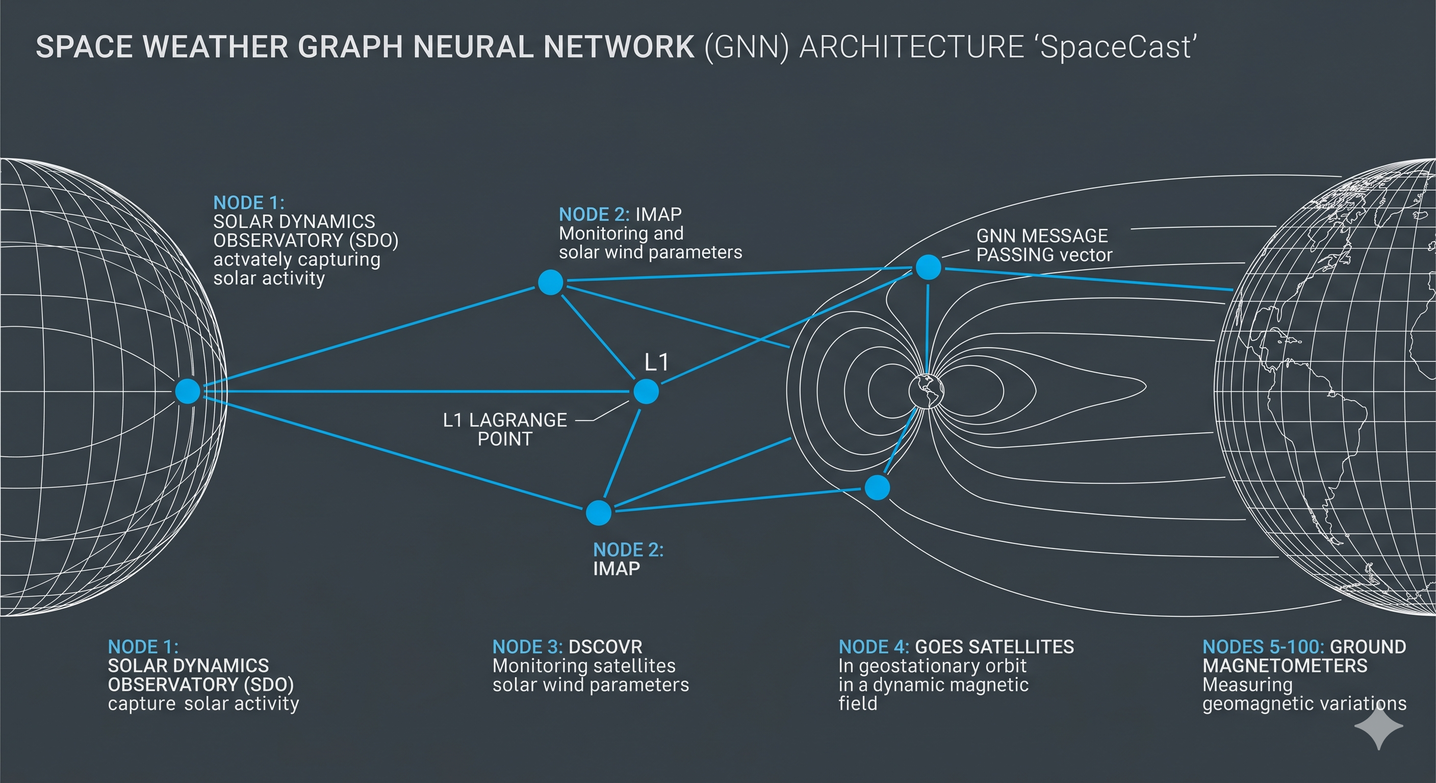
Space Weather Graph Neural Network (GNN) Architecture

The Spatial Network Nodes

Node 1 (The Source): Solar Dynamics Observatory (SDO) monitoring the Sun’s surface (Coronal Mass Ejection launch velocities).

Node 2 & 3 (The Upstream Sentinels): IMAP and DSCOVR at the L1 Lagrange point (measuring the kinetic lag and turbulence you just modeled).

Node 4 (The Earth Shield): GOES satellites in geostationary orbit (measuring the compression of Earth’s magnetosphere).

Nodes 5-100 (The Ground Impact): A global grid of ground-based magnetometers (measuring the actual induced electrical currents on Earth).

Systems Thinking

Heart Rate Variability (HRV)

By mapping the HRV framework to solar wind telemetry, the signal were seperated into macro-environmental shifts (SDNN, SD2, low-frequency power) and micro-turbulent noise (RMSSD, SD1). The high pNN(1.0) value (36.14%) indicates that classical smoothing algorithms might struggle with this data, as step-like jumps are highly characteristic of the local measurement environment.

By adapting cardiovascular metrics to space physics, we can map heart-rate concepts directly to plasma thermodynamics:

SDNN (Standard Deviation of Normal intervals): Maps to Macroscopic Volatility. It represents large-scale fluctuations in the bulk kinetic energy of the solar wind.
RMSSD (Root Mean Square of Successive Differences): Maps to Microscopic Turbulence. Because it measures the immediate jump from one 12-second reading to the next, it serves as a proxy for the plasma’s internal kinetic temperature and local entropy cascade.

Using K-Means clustering on 4-hour intervals, the HRV framework identifies three distinct thermodynamic states in the dataset:

1. The Laminar / Quiet State (Equilibrium)

HRV Profile: Extremely low SDNN ( $\approx 8.52$ ) and low RMSSD ( $\approx 1.04$ ).
Average Bulk Velocity: 394.8 $\text{ km/s}$
Thermodynamic Judgment: This represents a highly stable, adiabatic expansion phase of the slow solar wind. Because RMSSD is very low, there is minimal microscopic turbulence or internal heating occurring. The plasma flows smoothly outward from the sun in a relaxed thermodynamic equilibrium, devoid of sudden shocks or energy injections.

2. The Transitional State (Metastable)

HRV Profile: Moderate SDNN ( $\approx 17.32$ ) and elevated RMSSD ( $\approx 2.34$ ).
Average Bulk Velocity: 514.1 $\text{ km/s}$
Thermodynamic Judgment: This is a metastable boundary layer. The solar wind speed has increased significantly, likely due to a fast-wind stream catching up to a slower stream (a Co-rotating Interaction Region). The elevated RMSSD indicates increased particle collisions, local heating, and a rising degree of entropy. The plasma is actively negotiating a change in macroscopic kinetic energy.

3. The Highly Turbulent State (Non-Equilibrium / Shock)

HRV Profile: High SDNN ( $\approx 30.35$ ) and severe RMSSD ( $\approx 4.70$ ).
Average Bulk Velocity: 512.6 $\text{ km/s}$
Thermodynamic Judgment: This state represents a complete breakdown of laminar flow, indicative of a shockwave, sudden magnetic reconnection, or the turbulent wake of a Coronal Mass Ejection (CME).

The exceptionally high RMSSD means the microscopic energy cascade is violent—particles are scattering chaotically. Thermodynamically, this is a non-equilibrium state characterized by high local entropy, massive energy dissipation, and high effective kinetic temperatures.

Impact on Heart and Pacemakers?

Is there a connection between CME Events and HRV Data (if available)? Will not be part of this post. Or impacts on Pacemakers?

Synergetic (Herman Haken) – Self Organization

Synergetics is a deeply interdisciplinary theory of self-organization. It suggests that in complex, open systems (like space plasma and the solar wind), the chaotic, high-dimensional microscopic interactions “self-organize.” The behavior of the entire system becomes dominated by a very small number of slow-moving variables called Order Parameters.

The middle plot (Synergetic Potential Landscape) reveals a distinct, deep “well” (attractor state) around 640–645 km/s. In Synergetics, systems tend to roll down into the minima of the potential. This indicates that during this mission timeframe, the solar wind possessed a highly stable “metastable” state near 643 km/s. It was heavily anchored there, requiring a massive injection of external energy (like a Coronal Mass Ejection) to push the system out of this well. – To be validated.

The Carrington Event—the most powerful solar storm in history

In 1859, Earth was hit by the most powerful geomagnetic storm ever recorded. It was called the Carrington Event. It was caused by a coronal mass ejection (CME). A cloud of solar plasma reached the planet in just 17.6… pic.twitter.com/VwJUnhgqMh
— Black Hole (@konstructivizm) May 29, 2026

Data Selection – How to

https://cdaweb.gsfc.nasa.gov