Circular Astronomy
Twitter List – See all the findings and discussions in one place
-
The Mysterious Discovery of JWST That No One Saw Coming
Are We Inside a Cosmic Whirlpool? Recent JWST Advanced Deep Extragalactic Survey (JADES) observations of mysterious cosmological anomalies in the rotational patterns of galaxies challenge our understanding of the universe and reveal surprising connections to natural growth patterns.
The rotation of 263 galaxies has been studied by Lior Shamir of Kansas State University, with 158 rotating clockwise and 105 rotating counterclockwise. The number of galaxies rotating in the opposite direction relative to the Milky Way is approximately 1.5 times higher than those rotating in the same direction.
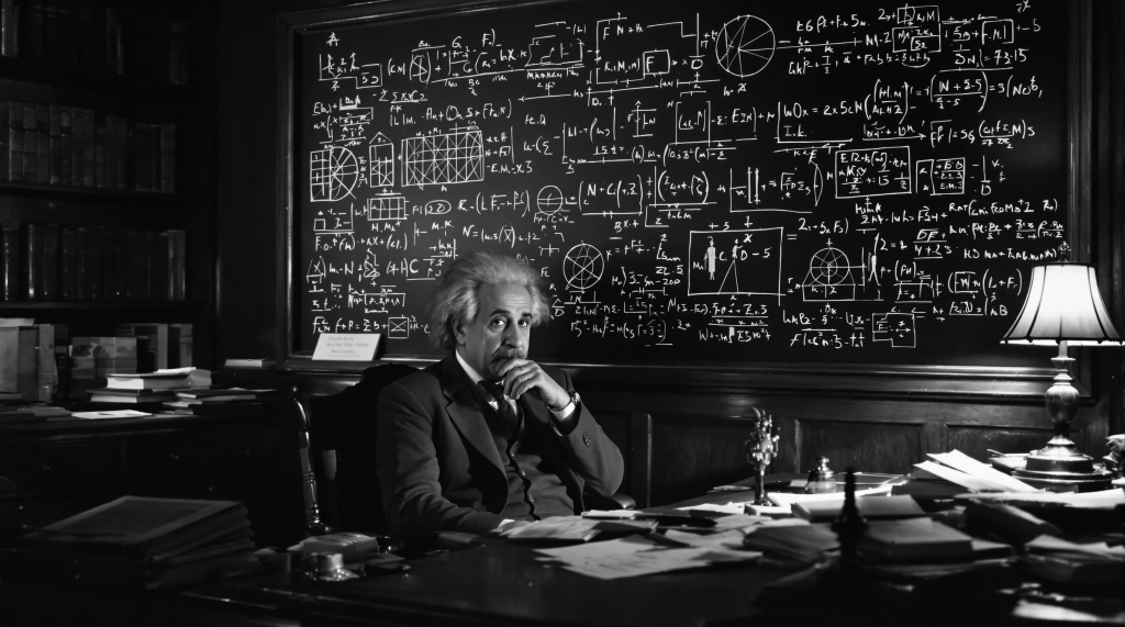
New Cosmological anomalies that challenge our cosmological models and would have angered Einstein.
This observation challenges the expectation of a random distribution of galaxy rotation directions in the universe based on the isotropy assumption of the Cosmological Principle.
This is certainly not something Einstein would have liked to hear during his lifetime, but it would have excited Johannes Kepler.
What does this mean for our cosmological models, and why would it make Johannes Kepler happy?
The 1.5 ratio in galaxy rotation bias is intriguingly close to the Golden Ratio of 1.618. The Golden Ratio was one of Johannes Kepler’s two favorites. The astronomer Johannes Kepler (1571–1630) referred to the Golden Ratio as one of the “two great treasures of geometry” (the other being the Pythagorean theorem). He noted its connection to the Fibonacci sequence and its frequent appearance in nature.

What is the Fibonacci sequence?
The Italian mathematician Leonardo of Pisa, better known as Fibonacci, introduced the world to a fascinating sequence in his 1202 book Liber Abaci (The Book of Calculation). This sequence, now famously known as the Fibonacci sequence, was presented through a hypothetical problem involving the growth of a rabbit population.

The growth of a rabbit population and why it matters?
Fibonacci posed the following question: Suppose a pair of rabbits can reproduce every month starting from their second month of life. If each pair produces one new pair every month, how many pairs of rabbits will there be after a year?

The solution unfolds as follows:
- In the first month, there is 1 pair of rabbits.
- In the second month, there is still 1 pair (not yet reproducing).
- In the third month, the original pair reproduces, resulting in 2 pairs.
- In the fourth month, the original pair reproduces again, and the first offspring matures and reproduces, resulting in 3 pairs.
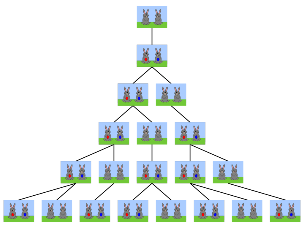
Image Source: https://commons.wikimedia.org/wiki/File:FibonacciRabbit.svg
This pattern continues, with each new generation adding to the total, where each term is the sum of the two preceding terms.
The Fibonacci sequence generated is: 1, 1, 2, 3, 5, 8, 13, 21, 34, 55, …
While this idealized model of a rabbit population assumes perfect conditions—no sickness, death, or other factors limiting reproduction—it reveals a growth pattern that approaches the Golden Ratio as the sequence progresses. The ratio is determined by dividing the current population by the previous population. For example, if the current population is 55 and the previous population is 34, based on the Fibonacci sequence above, the ratio of 55/34 is approximately 1.618.
However, in reality, the growth rate of a rabbit population would likely fall below this mathematical ideal ratio due to natural constraints.Yet, this growth (evolutionary) pattern appears quite often in nature, such as in the growth patterns of succulents.

The growth patterns in succulents often follow the Fibonacci sequence, as seen in the arrangement of their leaves, which spiral around the stem in a way that maximizes sunlight exposure. This spiral phyllotaxis reflects Fibonacci numbers, where the number of spirals in each direction typically corresponds to consecutive terms in the sequence.
Spiral galaxies exhibit a similar growth (evolutionary) pattern in their spiral arms.
Spiral galaxies, like the Milky Way, display strikingly similar growth patterns in their spiral arms, where new stars are continuously formed and not in the center of the galaxy.
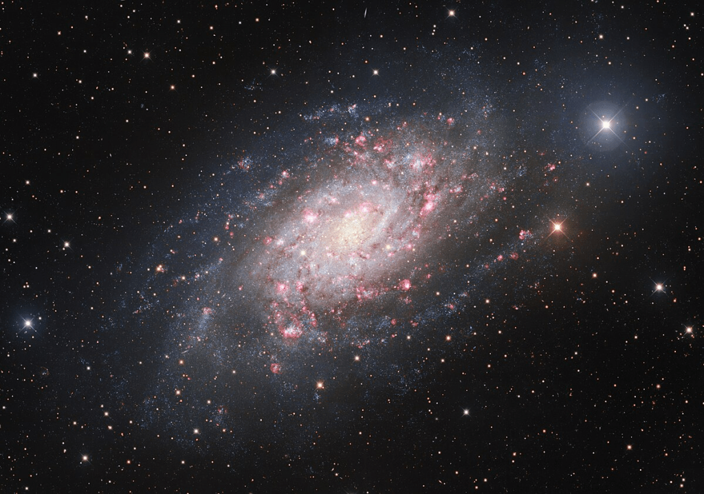
Image Source: https://commons.wikimedia.org/wiki/File:A_Galaxy_of_Birth_and_Death.jpg
Returning to the observations and research conducted by Lior Shamir of Kansas State University using the JWST.
The most galaxies with clockwise rotation are the furthest away from us.
The GOODS-S field is at a part of the sky with a higher number of galaxies rotating clockwise
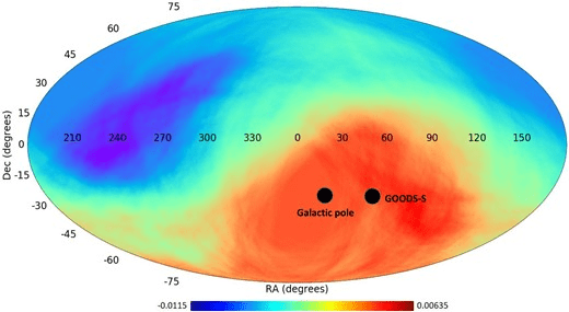
Image Source: Figure 10 https://doi.org/10.1093/mnras/staf292
“If that trend continues into the higher redshift ranges, it can also explain the higher asymmetry in the much higher redshift of the galaxies imaged by JWST. Previous observations using Earth-based telescopes e.g., Sloan Digital Sky Survey, Dark Energy Survey) and space-based telescopes (e.g., HST) also showed that the magnitude of the asymmetry increases as the redshift gets higher (Shamir 2020d).” Source: [1]“It becomes more significant at higher redshifts, suggesting a possible link to the structure of the early universe or the physics of galaxy rotation.” Source: [1]
Could the universe itself be following the same growth patterns we see in nature and spiral galaxies?
This new observation by Lior Shamir is particularly intriguing because, if we were to shift the perspective of our standard cosmological model—from one based on a singularity (the Big Bang ‘explosion’), which is currently facing a lot of challenges [2], to a growth (evolutionary) model—we would no longer be observing the early universe. Instead, we would be witnessing the formation of new galaxies in the far distance, presenting a perspective that is the complete opposite of our current worldview (paradigm).
NEW: Massive quiescent galaxy at zspec = 7.29 ± 0.01, just ∼700 Myr after the “big bang” found.
RUBIES-UDS-QG-z7 galaxy is near celestial equator.
It is considered to be a “massive quiescent galaxy’ (MQG).
These galaxies are typically characterized by the cessation of their star formation.
https://iopscience.iop.org/article/10.3847/1538-4357/adab7a
The rotation, whether clockwise or counterclockwise, has not yet been observed.Reference
The distribution of galaxy rotation in JWST Advanced Deep Extragalactic Survey
Lior Shamir
[1 ] https://academic.oup.com/mnras/article/538/1/76/8019798?login=false
The Hubble Tension in Our Own Backyard: DESI and the Nearness of the Coma Cluster
Daniel Scolnic, Adam G. Riess, Yukei S. Murakami, Erik R. Peterson, Dillon Brout, Maria Acevedo, Bastien Carreres, David O. Jones, Khaled Said, Cullan Howlett, and Gagandeep S. Anand
[2] https://iopscience.iop.org/article/10.3847/2041-8213/ada0bd
Reading Recommendation:
The Golden Ratio, Mario Livio, 2002
Mario Livio was an astrophysicist at the Space Telescope Science Institute, which operates the Hubble Space Telescope.
RUBIES Reveals a Massive Quiescent Galaxy at z = 7.3
Andrea Weibel, Anna de Graaff, David J. Setton, Tim B. Miller, Pascal A. Oesch, Gabriel Brammer, Claudia D. P. Lagos, Katherine E. Whitaker, Christina C. Williams, Josephine F.W. Baggen, Rachel Bezanson, Leindert A. Boogaard, Nikko J. Cleri, Jenny E. Greene, Michaela Hirschmann, Raphael E. Hviding, Adarsh Kuruvanthodi, Ivo Labbé, Joel Leja, Michael V. Maseda, Jorryt Matthee, Ian McConachie, Rohan P. Naidu, Guido Roberts-Borsani, Daniel Schaerer, Katherine A. Suess, Francesco Valentino, Pieter van Dokkum, and Bingjie Wang (王冰洁)
https://iopscience.iop.org/article/10.3847/1538-4357/adab7a
Appendix Spiral Galaxies:
Spiral galaxies are known for their stunning and symmetrical spiral arms, and many of them exhibit patterns that approximate logarithmic spirals, which are mathematically related to the Golden Ratio. While not all spiral galaxies perfectly follow the Golden Ratio, some exhibit spiral arm structures that closely resemble this pattern. Here are some notable examples of spiral galaxies with logarithmic spiral patterns:
1. Milky Way Galaxy
- Our own galaxy, the Milky Way, is a barred spiral galaxy with arms that approximate logarithmic spirals. The four primary spiral arms (Perseus, Sagittarius, Scutum-Centaurus, and Norma) follow a logarithmic pattern, though not perfectly aligned with the Golden Ratio.
2. M51 (Whirlpool Galaxy)
- The Whirlpool Galaxy is one of the most famous examples of a spiral galaxy with well-defined logarithmic spiral arms. Its arms are nearly symmetrical and exhibit a pattern that closely resembles the Golden Ratio.
3. M101 (Pinwheel Galaxy)
- The Pinwheel Galaxy is a grand-design spiral galaxy with prominent and well-defined spiral arms. Its structure is often cited as an example of a logarithmic spiral in astronomy.
4. NGC 1300
- NGC 1300 is a barred spiral galaxy with a striking logarithmic spiral pattern in its arms. It is often studied for its near-perfect spiral structure.
5. M74 (Phantom Galaxy)
- The Phantom Galaxy is another grand-design spiral galaxy with arms that follow a logarithmic spiral pattern. Its symmetry and structure make it a textbook example of this phenomenon.
6. NGC 1365
- Known as the Great Barred Spiral Galaxy, NGC 1365 has a prominent bar structure and spiral arms that exhibit a logarithmic pattern.
7. M81 (Bode’s Galaxy)
- Bode’s Galaxy is a spiral galaxy with arms that follow a logarithmic spiral structure. It is one of the brightest galaxies visible from Earth and a popular target for astronomers.
8. NGC 2997
- This galaxy is a grand-design spiral galaxy with arms that closely resemble logarithmic spirals. It is located in the constellation Antlia.
9. NGC 4622
- Known as the “Backward Galaxy,” NGC 4622 has a unique spiral structure with arms that follow a logarithmic pattern, though its rotation direction is unusual.
10. M33 (Triangulum Galaxy)
- The Triangulum Galaxy is a smaller spiral galaxy with arms that exhibit a logarithmic spiral structure. It is part of the Local Group, along with the Milky Way and Andromeda.
-
How to Download, View, And Edit Images from the James Webb Space Telescope with Jdaviz and Imviz
Like to comfortably view and edit images from the Jamew Webb Space Telescope like an astronomer ?
Then follow this step by step cheatsheet guides if you are using windows on a PC .
Main Software Components
There are three key software components required:
- Microsoft C++ 14
- Jupyter Notebook (Python)
- Jdaviz
Additonal
- MAST Token to be able to download the images with Imviz.
Prerequsites:
Microsoft Visual C++ 14.0 or greater

error: Microsoft Visual C++ 14.0 or greater is required If Microsoft Visual C++ 14.0 or greater is not installed, the installation of Jdaviz will fail. Without Jdaviz the downloaded images from the James Webb Space Telescope cannot be edited.
How to install Microsoft Visual C++
- Navigate to: https://visualstudio.microsoft.com/downloads/
- Download Visual Studio 2022 Community version
- Follow the instructions in this post: Install C and C++ support in Visual Studio | Microsoft Docs

Cheatsheet: Install Visual Studio 2022 MAST Token
- Navigate to https://ssoportal.stsci.edu/token
If you do not have not an account yet, please follow below steps to create your account:
- Click on the Forgotten Password? link
- Enter your email Adress
- Click Send Reset Email Button
- Click Create Account Button
- Click Launch Button
- Enter the Captcha
- Click Submit Button
- Enter your email
- Click Next Button
- Fill in the Name Form
- Click Next Button
- Fill in the Insitution (e.g. Private Citizen or Citizen Scientist)
- Click Accept Institution Button
- Enter Job Title (whatever you are or like to be ;-))
- Click Next Button
- New Account Data for your review is presented, in case of missing contact data, step 17 might be necessary
- Fill in Contact Information Form
- Click Next Button
- Click Create Account Button
- In your email account open the reset password emal
- Click on the link
- Enter Password
- Enter Retype Password
- Click Update Password
- Navigate to https://ssoportal.stsci.edu/token
- Now log on with your email and new account password
- Click Create Token Button
- Fill in a Token Name of your choice
- Click Create Token Button
- Copy the Token Number and save it for later use in Imviz to download the images from the James Webb Space Telescope
Quite a lot of steps for a Token.

Cheatsheet: Create MAST Account 
Cheatsheet: Set Passord for new Account 
Cheatsheet: Create MAST Token for use in Imviz Jupyter Notebook
Jupyter notebook comes with the ananconda distribution.
- Navigate to: https://www.anaconda.com/products/distribution#windows
- Follow the instructions at: https://docs.anaconda.com/anaconda/install/windows/
Install Jdaviz
- Navigate to: Installation — jdaviz v2.7.2.dev6+gd24f8239
- Open the Jupyter Notebook
- Open Terminal from Jupyter Notebook
- Follow the instruction in: Installation — jdaviz v2.7.2.dev6+gd24f8239
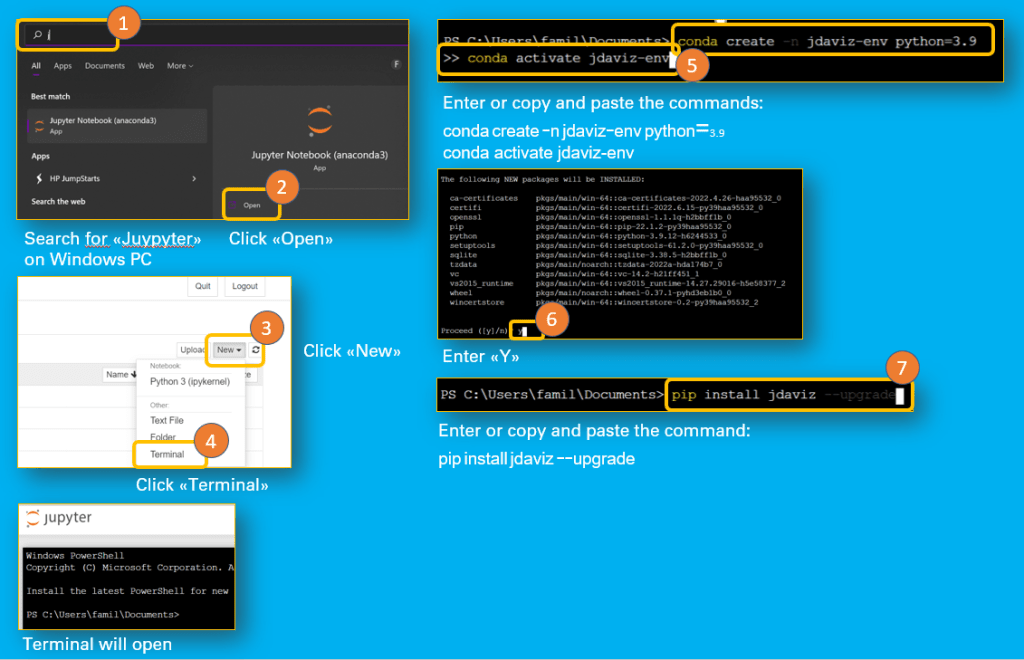
Cheatsheet: Install Jdaviz How to use IMVIZ
Imviz is installed together with Jdaviz.
Following steps to take in order to use Imviz:
- Navigate to: GitHub – orifox/jwst_ero: JWST ERO Analysis Work
- Click Code Button
- Click Download Zip
- If you do not have unzip, then the next steps might work for you:
- In Download Folder (PC) click the jwst_ero master zip file
- Then click on the folder jwst_ero master
- Copy file MIRI_Imviz_demo.jpynb
- Paste the file in the download folder
- Open Jupyter notebook
- Click Upload Button
- Select the file MIRI_Imviz_demo.jpynb
- Click Open Button
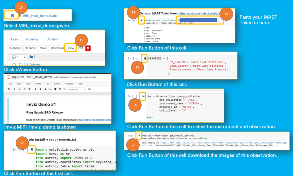
- Select the file MIRI_Imviz_demo.jpynb in the Jupyter Notebook file list
- Click View Button
- Click Run Button First Cell
- Paste MAST Token in next cell
- Click Run Button of this Cell
- Click then Run Button of next Cell
- Click Run Button of the following Cell
- Click Run Button of the next Cell to download the images
- Copy the link to the downloaded image file
- Past link into the First Cell in 3. Load and Manipulate Data
- Do the same in the next Cell
- Click Run Button of the Cell to open Imviz
- Click Run Button on the next Cell to load images in Imviz

Cheatsheet: Upload MIRI_Imviz_demo.jpynb in Jupyter notebook Now all set to download the images of the JWST observation:
Cheatsheet: Download JWST images with Imviz And now all is set to open and edit the images in Imviz
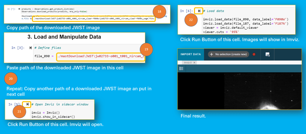
Cheatsheet: Open Images in Imviz And finally you are ready to follow the video tutorials in order to learn how to use Imviz to manipulate the JWST images.
Video Tutorials for Imviz:
And this is the master Ori Fox of the Imviz demo notebook file if you like to follow him on Twitter
-
Time for a new scientific debate – Accretion vs Convection
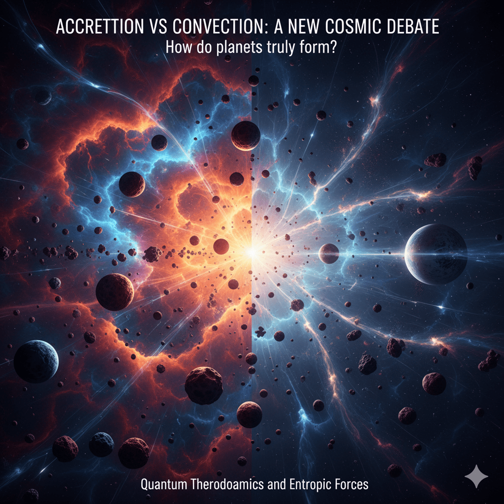
To what degree is gravity needed to form structures in space? While many believe that celestial bodies (stars, planets, moons, meteoroids) can only form through gravitational attraction in the vacuum of space, I believe that these bodies form through a thermodynamic process similar to the formation of hydrometeors (e.g., hail). This is because our solar system possesses a boundary layer, a discovery made by the Interstellar Boundary Explorer (IBEX) mission in 2013.
In simple terms: Planets, moons, and small bodies are formed within convection cells created by the jet streams of a young sun, under the influence of strong magnetic fields.
Recently, a new paper introduced quantum models in which gravity emerges from the behavior of qubits or oscillators interacting with a heat bath.
More details and link to the research paper: On the Quantum Mechanics of Entropic Forces
https://circularastronomy.com/2025/10/09/entropic-gravity-explained-how-quantum-thermodynamics-could-replace-gravitons/ -
What Einstein, Newton and Kepler Did not Know About the Solar System During Their Lifetime
Kepler
When Kepler established the first theory and three principles of our solar system he could describe the movement of the planets around the sun but he could not explain why these planets would not vanish in the void around the solar system. He assumed magnetic fields to be the tether to hold our planets in place.
Newton
No evidence was found for these super magentic fields between the sun the planets. Later Newton used his gravity concept to explain the movement of the planets. And this was quite successful. Yet the movement of Mercury could not be explained completly with the gravity concept of Newton.
Einstein
It was Einstein’s Relativity Theory that could well explain the movement of mercury.
What They Did Not Know
But what they did not know at that time: The solar system has a boundary – the IBEX Ribbon. There is a clear distinction between the solar system (heliosphere) and the interstellar space. It is the heliospheric boundary layer (HBL) with decreased plasma density and draped magnetic field.
The Interstellar Boundary Explorer (IBEX) discovered the IBEX Ribbon, a structure beyond the heliopause in the very local interstellar medium (VLISM). This Ribbon was unexpected and not predicted by any prior theory or model.
“The interstellar medium (ISM) of our Galaxy is magnetized, compressible and turbulent, influencing many key ISM properties, such as star formation, cosmic-ray transport, and metal and phase mixing.” Reference: The spectrum of magnetized turbulence in the interstellar medium
Would they have reconsidered their theory if they would have had this knowledge by then?
On the right and left side of the IBEX spacecraft (round golden ring) are each the IBEX high and low single pixel sensors. IBEX High measures ENA (Energy Neutral Atoms) 400 eV to 6 keV and the IBEX Low measures between 10 eV to 2 keV. Solar System
“Our solar system is located between the Perseus and Carina-Sagittarius spiral arms of the Galaxy at the inner edge of the Orion Spur, some 28,000 light years from the galactic center”
Reviews of Geophysics – 2013 – McComas – IBEX s Enigmatic Ribbon in the sky and its many possible sources
IBEX Ribbon
The IBEX Ribbon is a fascinating and unexpected discovery made by NASA’s Interstellar Boundary Explorer (IBEX) spacecraft in 2009. It is a bright, arc-like feature observed in the first all-sky map of energetic neutral atoms (ENAs) beyond our solar system. The ribbon is located near the heliopause, where the Sun’s influence gives way to incoming interstellar particles. The name was suggested in 2009 by Christina Prested, then a graduate student at Boston University.
Key characteristics of the IBEX Ribbon:
- Density: The ribbon is three to six times denser than expected, consisting of fast-moving ENAs coming towards Earth.
- Location: It is situated at the edge of our solar system, near the boundary between the heliosphere and interstellar space.
- Formation time: The process that creates the ribbon particles takes approximately 3-6 years.
Theories about the IBEX Ribbon’s origin:
- Solar wind interaction: Many scientists believe the ribbon results from solar wind particles encountering the galaxy’s magnetic field, which reflects them back towards us.
- Reflected solar material: One prominent theory proposes that the ribbon particles are actually solar material reflected back after a long journey to the edges of the Sun’s magnetic boundaries.
Significance of the IBEX Ribbon:
- Interstellar magnetic field: The ribbon provides information about the strength and direction of the magnetic field outside the heliosphere, offering insights into our galactic neighborhood.
- Heliosphere interaction: It helps scientists understand how our space environment interacts with the interstellar environment beyond the heliopause.
Ongoing research:
Scientists continue to study the IBEX Ribbon, developing more sophisticated models and analyzing its evolution over time. The ribbon exhibits gradual and continuous changes, and researchers are working to better understand its structure and origins.
References:
https://www.astronomy.com/observing/weird-object-the-ibex-ribbon/
https://www.nasa.gov/missions/ibex/nasas-ibex-observations-pin-down-interstellar-magnetic-field/
https://agupubs.onlinelibrary.wiley.com/doi/full/10.1002/2013RG000438 -
Einstein’s Glitch in Gravity
https://iopscience.iop.org/article/10.1088/1475-7516/2024/03/045
Robin Y. Wen1,2, Lukas T. Hergt3, Niayesh Afshordi4,5,6 and Douglas Scott3
Gravity on large scales is weaker by roughly 1 Percent.
Citation:
“Additionally, we find that roughly one percent weaker superhorizon gravity can somewhat ease the Hubble and clustering tensions in a range of cosmological observations, although at the expense of spoiling fits to the baryonic acoustic oscillation scale in galaxy surveys.”
“we discuss how future observations may elucidate this potential cosmic glitch in gravity, through a four-fold reduction in statistical uncertainties”
Remark:
Reminds me of the Pauli and Bohr discussion about the existence of the neutrino: Bohr as well used statistics as argument against the neutrino.
-
Bennu Samples 1 Percent Analysed – Chondrules or CAI (Calcium-Aluminum-Inclusion) This is the Question
Citation from article:
Harold Connolly Jr., a meteorite expert at Rowan University.
Sara Russell, a meteorite researcher at the Natural History Museum in London
Meteorite experts Loan Le and Kathie Thomas-Keprta at the Johnson Space CenteChondrules formed when small grains of dust were heated early on in the solar system and later cooled.
“Chondrules are so unusual,” says Thomas-Keprta. “They would never have been predicted if they didn’t exist.”
Could be a reference for: https://circularastronomy.com/planet-and-comet-formation-process-in-convection-cell-rings/

-
Rocky Exoplanet 55 Cancri e Has an Atmosphere
James Web Telescope discovered atmospheric gases. 55 Canceri e is 41 light years away from earth. Dayside temperature is 2200 Celsius.
Furhter research required into the conditions that make it possible for such a hot rocky planet to sustain a gas-rich atmosphere. One such condition could be magnet fields.
Researchers:
Renyu Hu, Aaron Bello-Arufe, Michael Zhang, Kimberly Paragas, Mantas Zilinskas ,Christiaan van Buchem, Michael Bess, Jayshil Patel, Yuichi Ito, Mario Damiano, Markus Scheucher, Apurva V. Oza, Heather A. Knutson, Yamila Miguel, Diana Dragomir, Alexis Brandeker & Brice-Olivier Demory
A secondary atmosphere on the rocky Exoplanet 55 Cancri e
-
Black Hole Sagittarius A Acts Like a Galactic Center Chimney for Plasma Outflows
https://arxiv.org/abs/2310.02892
Using NASA’s Chandra X-ray Observatory, astronomers have identified an exhaust vent attached to a “chimney” of hot gas near the center of our Milky Way galaxy. This chimney and exhaust vent are located around the supermassive black hole known as Sagittarius A* (or Sgr A* for short).
Researchers: Scott C. Mackey, Mark R. Morris, Gabriele Ponti, Konstantina Anastasopoulou, Samaresh Mondal
The authors see it as a result of a sequence of accretion events.
Further research required to determine other non-gravitational factors involved or more decisive.
-
Quantum Computing For Beginners – First Program in Less Than a Minute
The fastest way to learn quantum computing is to do it and then reflect and learn from the experience. The IBM Composer is the ideal way to start for a Novice. No need to install Qiskit and Python and spent a lot of time getting connected to one of the IBM Quantum Computers.
Just follow the 9 steps in the quick guide cheat sheet below:
Quick Guide Cheat Sheet First Program Let’s build your first quantum program on IBM Quantum Composer!
1. Head to your IBM Quantum Learning account: https://quantum.ibm.com/composer
2. Pick a gate: Think of gates as tools that manipulate Qubits (Classical Computer Bits = 0 or 1). In this example, we’ll use the “RZ” gate.
3. Drag the “RZ” gate to the first Qubit line. This puts the Qubit in a special state called superposition, like a coin spinning in the air (both heads and tails at the same time!).
4. Add a measurement: Drag the “Measure” icon to the same Qubit line. This lets us see the outcome of the program.
5. Run the program! You can choose a real quantum computer (like the one in Brisbane, Australia) or a simulator.
6. Wait your turn! Since the computer is shared, there might be a waiting queue for your program to run. You can check the status on the left panel.
Reflection
Reflecting on the first experience with quantum computing might lead to some of the following questions:
Why so many measurements (100) and not just 1 when you run the program on the IBM Quantum computer ?
Notice the many icons in the Operations block of the IBM Composer interface? Are all these quantum gates like the RZ gate besides the icon for measurement? What is their purpose?
What are Qubits and why only 4 Qubits?
What is the c line below the Qubits that the measure icon is pointing to with a line?
What does RZ Gate stand for?
First let’s take a look at the results:
Quantum Computing Results Quick Guide Cheat Sheet Check your results:
After running the program and measuring repeatedly for 100 times the results show a probability above 100% for the bit value of 0 and a negativ probability for a bit value of 1!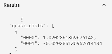
Negativ probability of 0.02 (2%)
Welcome, you are entering a world where your everyday intuition will not work. And you are not alone. Not even Albert Einstein based on his scientific intuition could accept quantum mechanics as a complete theory during his lifetime.
In this first program only one RZ gate was created. What would happen to the negativ probability if more RZ gates are usded?

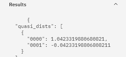
The negativ probability increased to over 4%.
This is even more strange as the probability before computing was calculated to be 100% for zero (0) by the IBM Qunatum Composer in the Probabilities pane:
View Probability before running Quantum Program Could it be that the measuring system of the IBM Quantum Computer in Brisbane, Australia has a defect?
Let’s run the same program at the IBM Quantum Computer in Osaka, Japan.

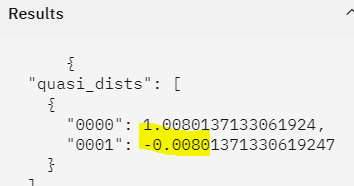
Different result, but still a negativ probability. Does it mean IBM Osaka has a better quantum computer than IBM Brisbane?
Probably not. Let’s run the same quantum program again at the IBM Brisbane Quantum Computer. Voilà:
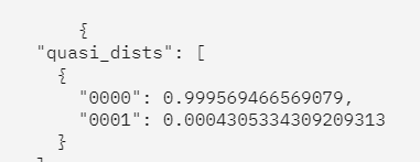
A new result and this time no negativ probability. In 99.95% cases the measurement got you a 0 as predicted but not all. Get used to the noise. Many see it as an error and want to correct it but there are a few scientist who see as a benefit of quantum computing.
First Principle: Quantum Computing is counterintuitive and noisy.
-
JWST Live Stream
-
Using State-of-the-Art Problem Solving for the Navier-Stokes Equations
Update 06.09.2025: Conceptual Witepaper on the plan to solve the millenium prize problem.
Do you believe that only mathematicians can solve these problems?
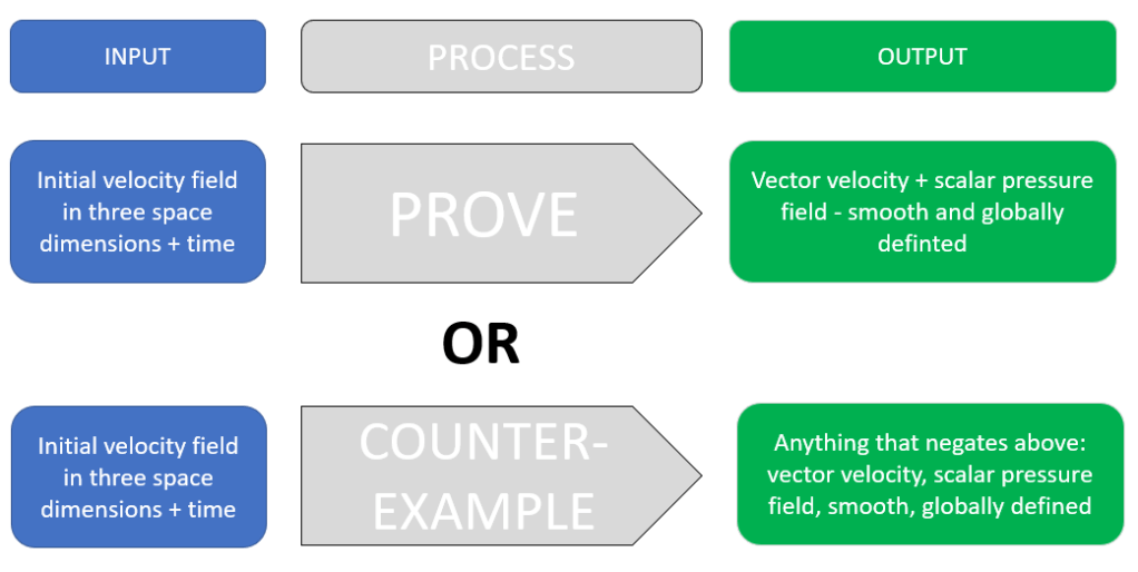
The Clay Mathematics Institute of Cambridge, Massachusetts (CMI) set out a million dollar prize in May, 2000 for anyone to:
Prove or give a counter-example of the following statement:
In three space dimensions and time, given an initial velocity field, there exists a vector velocity and a scalar pressure field, which are both smooth and globally defined, that solve the Navier-Stokes equations.
The incompressible Navier-Stokes equations are given by – Official Problem Description:
- Momentum equation (conservation of momentum): ∂t∂u+(u⋅∇)u=−∇p+νΔu+f, where:
- u=u(x,t) is the velocity field of the fluid,
- p=p(x,t) is the pressure field,
- ν>0 is the kinematic viscosity,
- f=f(x,t) is the external force per unit volume,
- x∈R3 is the spatial coordinate,
- t≥0 is time.
- Continuity equation (incompressibility condition): ∇⋅u=0.
The Millennium Prize Problem asks whether, for smooth initial conditions u0(x) satisfying ∇⋅u0=0, there exists a globally defined, smooth solution u(x,t) and p(x,t) for all t>0. Alternatively, it asks whether singularities (blow-ups) can form in finite time.
The first counterintuitive approach in state-of-the-art problem-solving is to step back and resist the urge to immediately jump into finding solutions. Instead, the key focus should be on understanding and analyzing the problem.
Navier-Stokes: https://circularastronomy.com/2025/08/23/the-fastest-way-to-understand-any-mathematical-function/
There are many ways to go about problem solving
The idea is to ask the most effective and least amount of questions in optimal sequence to extract as much information as possible.
Major questions to ask before starting the problem-solution process:
- How much time is available to solve the problem?
- What is the environment surrounding the problem?
- What is the current state of the problem?
- Are there alternative problems to consider?
- Have these alternative problems been solved yet?
Using Systems Thinking to Approach the Problem
Solving a system’s problem in nature:
The first step in systems thinking is to look outside the system. What larger system is it a part of? What is the surrounding environment?
Navier Stokes equation are part of classical mechanics and are derived from applying Newton’s second law of motion to fluid motion.
Navier-Stokes equations are widely used in engineering, meteorology, oceanography, and astrophysics to model phenomena like air flow over an airplane wing, weather patterns, ocean currents, and even the behavior of stars.
The key is to establish system boundaries in order to analyze the system itself. System boundaries define the systems properties. The following questions can help identify these boundaries.
What is a FlUID and when it is not a FLUID?
First, describe the distinction between fluid and non-fluid in natural language, and then use mathematical abstractions to define these concepts.
Fluids are substances that flow and take the shape of their container. Fluids can be liquids or gases. Plasma is also a fluid, but it is not covered by the Navier-Stokes Equation.
Archimedes, a Greek mathematician and engineer, laid the foundation for fluid mechanics with his discovery of buoyancy. His famous principle states that an object submerged in a fluid experiences an upward force equal to the weight of the displaced fluid.
Al-Khazini and Al-Biruni expanded on Archimedes’ work. They studied fluid density, pressure, and hydrostatics, applying these principles to engineering and astronomy.
Leonardo da Vinci (1452–1519): Da Vinci studied the motion of water and air, observing turbulence, vortices, and wave patterns. He sketched detailed diagrams of fluid flow, laying the groundwork for modern fluid dynamics.
Evangelista Torricelli (1643): Torricelli invented the barometer and demonstrated that air has weight, leading to the study of atmospheric pressure.
Blaise Pascal (1653): Pascal formulated the principle of fluid pressure, stating that pressure applied to a confined fluid is transmitted equally in all directions (Pascal’s Law).
Daniel Bernoulli (1738): Bernoulli’s Principle, published in Hydrodynamica, describes how fluid pressure decreases as its velocity increases.
Leonhard Euler (1757): Euler developed the Euler equations, which describe the motion of ideal (non-viscous) fluids.
Claude-Louis Navier (1822) and George Gabriel Stokes (1845): They extended Euler’s work by incorporating viscosity, leading to the Navier-Stokes equation, which describes the motion of real (viscous) fluids.
Osborne Reynolds (1883): Reynolds studied the transition between laminar (smooth) and turbulent (chaotic) flow, introducing the Reynolds number, a dimensionless quantity that predicts flow behavior.
Ludwig Prandtl (1904): Prandtl introduced the concept of the boundary layer, explaining how fluid flows near surfaces like airplane wings.
When Is a Substance Not a Fluid?
Solids resist deformation and maintain a fixed shape under shear stress. Some materials, like rubber or clay, can deform under stress but do not flow continuously. Glass is sometimes called an “amorphous solid” because it behaves like a solid on short timescales but flows extremely slowly over long timescales. Substances like sand or grains can flow under certain conditions (e.g., in an hourglass), but they are not true fluids because their flow depends on particle interactions rather than continuous deformation.
Non-Newtonian Solids: Some materials, like oobleck (a cornstarch-water mixture), behave like a solid under certain conditions (e.g., when struck quickly) and like a fluid under others. These are complex materials that blur the line between solids and fluids.What is incompressible and when is it not?
First, describe the distinction between liquid and non-liquid in natural language, and then use mathematical abstractions to define these concepts.
What is a incompressible fluid and when it is not?
First, describe the distinction between liquid and non-liquid in natural language, and then use mathematical abstractions to define these concepts.
What is motion and when it is not?
First, describe the distinction between liquid and non-liquid in natural language, and then use mathematical abstractions to define these concepts.
See also hydrostatics (fluids at rest) : Archimedean screw
Based on the answers above, analyze existing mathematical papers on the Navier-Stokes equation and the Millennium Prize Problem.
In the next step, focus on examining the system itself, including its underlying paradigms.
Use natural language to describe the incompressible Navier-Stokes equation:
Imagine you are observing a fluid, like water or air, moving through space.
The change in velocity over time (how the fluid speeds up or slows down) is caused by:- The fluid carrying itself along,
- Pressure differences pushing the fluid,
- Viscosity smoothing out the motion
- External forces acting on the fluid.
At every point in the fluid, there is a velocity that tells you how fast and in what direction the fluid is moving.
This velocity changes over time and space.
What we want to understand what causes these changes.
- Start by looking at how the velocity at a point changes over time. “How does the speed and direction of the fluid at this spot evolve as time passes?”
- Consider how the fluid’s movement at one point is influenced by the movement of the fluid around it.
Imagine a river: the water at one spot is pushed along by the water upstream. - Pressure is like a force that pushes the fluid from areas of high pressure to areas of low pressure. If there’s a difference in pressure between two points, the fluid will accelerate toward the lower-pressure area.
- Viscosity is like the fluid’s internal resistance to motion. Imagine honey versus water: honey resists motion more because it’s more viscous.
- External forces. These could be things like wind pushing it sideways. These forces add to the motion of the fluid.
What you notice in the above descriptions is that they only consider the unidirectional flow of an incompressible liquid from a specific point onwards.
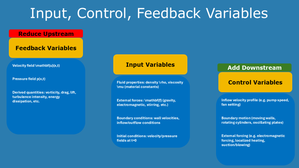
Input – Output Relationship
Another perspective involves analyzing the input-output relationship of the problem statement.
Remark: Systems Thinking was established in the 1940s and unknown to Navier and Stokes.
System rules define the systems behaviour (dynamic) and the behaviour defines and shapes the structure of the system. Vice versa the system boundaries and the environment influence the system rules and thus the behaviour. It is an oscillating interaction.
Polya’s problem solving technique in mathematics:
Polya’s approach is to start with a best guess.
Most mathematicians tend to believe that the Navier-Stokes equations will likely be proven to have smooth and globally defined solutions under the given conditions, rather than a counterexample being found.
If you examine the input-output relationship of the problem statement, the best guess seems to favor finding a counterexample rather than a proof. A likely starting point could be to search for a counterexample first, rather than attempting to prove it outright.
Let’s find out with a poll: https://strawpoll.com/XOgONlrOrn3
Backwards problem solving:
Rapid problem analysis
Inventive problem solving:
Use of AI Tools
Javier Gómez Serrano (Mathematician Brown University) teamed up with Google DeepMind Team. The team consists of 20 people who have been working on the solution for three years. On the team are two geophysicists — Ching-Yao Lai and Chinese Yongji Wang, authors of complex models for calculating melting ice in Antarctica — and additional two mathematicians: Tristan Buckmaster and Gonzalo Cao Labora.
Their attempt seems to target the boundary condition between solid and fluid.
My plan to win the Millenium prize with OpenAI:
Use the wisdom of the crowd
a) Internet searches
b) Citizen Research Communities
Use Analog Computing
Viktor Schauberger Waterflow
- Vortex geometry (spirals, implosions) might stabilize flows.
- In Navier–Stokes terms, this is equivalent to geometric alignment of vorticity — exactly one of the overlooked pieces in current approaches.
Christine Sindelar publications: https://www.researchgate.net/profile/Christine-Sindelar
Conceptual Witepaper on the plan to solve the millenium prize problem.
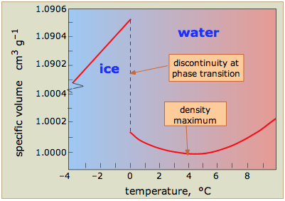
Interplay between two opposing aspects
Temperature of 273.16 K (0.01∘ C) and a partial vapor pressure of 611.657 Pa (approximately 0.006 atm).4 Below this pressure, liquid water cannot exist in a stable state. Any increase in temperature at a constant pressure below the triple point will cause ice to bypass the liquid phase and transition directly to vapor through the process of sublimation.3
Another critical state point is the critical point, where the liquid-gas boundary terminates and the two phases become indistinguishable, forming a supercritical fluid.2 For water, this occurs at a temperature of 647.096 K and a pressure of 22.064 MPa.2
A seminal study by Cheng and Lin in 2007 investigated the morphological changes of water within a vacuum cooling system, providing a precise timeline of the process.9 Their experiments showed that as the pressure in the chamber was reduced, a series of distinct events occurred: the liquid water began to produce tiny bubbles after 115.2 s, which grew larger at 121.2 s, leading to rapid boiling at 126.7 s. After the boiling subsided, the water entered the freezing stage at 181.5 s. The final ice mass, observed after 480 s, was found to have a two-layered structure: an irregular, porous layer on top and a dense layer below.9
Timeline Stages:
- 115.2 s – Bubble Formation
- 121.2 s – Larger Bubbles
- 126.7 s – Rapid Boiling
- 181.5 s – Freezing Begins
- 480 s – Final Ice Structure (Porous top layer, dense bottom layer)
laboratory experiments: a volume of water in a vacuum chamber with an insulating glass beaker is more likely to freeze than one in a conductive copper vessel, as the latter can more efficiently transfer ambient heat to the water, aiding the sublimation process after the initial freeze.6
Interplay between steepness and smoothness (Neither can be infinite or 0 in a liquid). Can be extended to the interplay of velocity and pressure (Either of it infinite or 0 will lead to no boundary layer, and no boundary layer means no liquid)
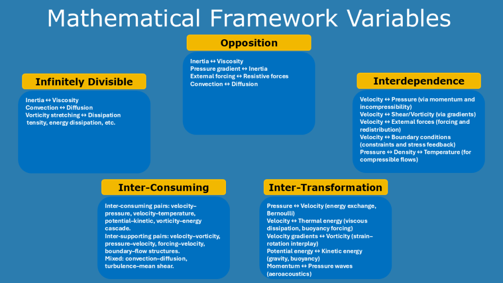
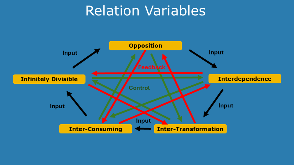
5 Postulates for Systems (Structural and Dynamic Aspects)
- Opposition: Two opposing aspects will restrict the other through opposition.
- Interdependence: Neither aspect can exist in isolation, without one there is no other and vice versa. Each aspect is the condition for the other’s existence. (Example Vacuum – no pressure no liquid)
- Inter-consuming-supporting: Continuous mutual-consumption and support between the two aspects. (Quantative change)
- Inter-transforming: In certain circumstances, either of the two aspects will transform into its opposite (Qualitive change). Extreme states of one of the aspects will eventually transform in the opposite. (Example Vacuum – part will turn into steam part into ice)
- No fundamental indivisible unit exists: Aspects are infinite divisble.
Mathematical frameworks (Dialectic dynamical inter-consuming systems)
Opposition: projective geometry, category theory, or optimization theory
Interdependence: dynamical systems (e.g. Heisenberg uncertainity principle), game theory, network theory
Inter-consuming-supporting: Lottka-Volterra(predator-prey)
Inter-transforming: nonlinear dynamics (laminar to turbulent flow), thermodynamics in vacuum, catastrophe theory (René thom)
No fundamental indivisible unit: Self similarity – Fuzzy Logic Fractal
Quantum Tornadoes
Generate Solution Options
What solution options have been published so far
Mathematical Concepts:
Nodes – (see Non Linear Equations in Differential Equations with Applications and Historical Notes – George F. Simmons Page 538: Figure 86 ) A critical point is called a node.
Solving Problems in Groups (Discord)
- Momentum equation (conservation of momentum): ∂t∂u+(u⋅∇)u=−∇p+νΔu+f, where:
-
A Method for Reading Scientific Abstracts with Lack of Time and Energy
The Abstract is the condensed version of a scientific paper. The target audience is the senior research community in the same field. Thus the vocabulary is complex and for novices and outsiders usually not understandable. It feels like visiting a huge buzzling foreign city for the first time without a map and trying to find the way to the hotel without knowing the local language and not understanding the street signs.
It takes great effort at the beginning to extract value from reading abstracts and doing so persistently. As an outsider in this research area and with many other commitments elsewhere I need an effective and efficent method to read and digest scientific abstracts despite time and mental energy constraints.
This method helps me to stay on course even in the worst and busiest moments.
I demonstrate the method on a concrete example.

Example: A Radiative-Convective Model for Terrestrial Planets with Self-Consistent Patchy Clouds
Read the last sentence of the abstract first (Update 17 August 2024)
It will summarize the key result of the paper
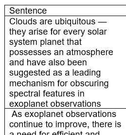
Tip from Dr. Andy Stapleton Break the abstract into single sentences.
I copy the abstract into word and then use convert text to table with the sentence point as delimeter and number of rows 1.
The result looks like this
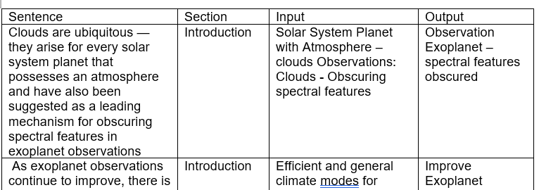
To the initial table I add three more rows. The first row is labled section, the second row input and the third row output.
If I have two spare minutes or more, I can return to the table at any time and continue the analysis; sentence by sentence.
Identify the sections – Introduction, Result, Discussion
Scientific papers usually have similar structures, but I always check before I fill in the section column. And usually I follow a certain sequence which is not from top of the table to the bottom.
In the first step I will identify all the sentences that would belong to the introduction section of the paper. Next I would go to the end of the table and assign all the rows that belong to the result and the discussion section.
Define the Output then Input per sentence
Each sentence usually has an output and an input content. In this step I will go back to the sentences that are part of the introduction and will start my output – input analysis; in this order. I always look for the output first before defining what the input is.
In my concrete example the output is “Exoplanet observations with obscured”- (meaning: keep from being seen like gray cloud obscuring the sun) – “spectral features”. While I note down the output I might immediately decypher complex vocabulary, that I do not yet fully understand and replace it with easier words.
Once done with the sentences of the introduction I would jump to the section results, discussion and/or conclusion and work through it the same way as in the introduction.
As you have noticed by now the largest part, the method section will come last. The method section is mainly relevant for those readers who want to replicate the results of the research paper. Often the method section can be skipped.
Highlighting words in the abstract
Additionally I would check the title and where in the abstract the terms or words in the title are mentioned. The same I will do for the key words and highlight those in the table as well.
In the final step I will prepare all these structured information for my visual brain. Usually it is easier and faster to remember visuals and patterns then concepts and text. So for every output I will identify visual representation and I might as well do it for the input factors. One place to start is in the paper itself but if it is not sufficient I would turn to Google Image search or use AI such as Stable Diffusion to generate visuals. The key driving question to identify those visuals is, what are the key figures, images, pattern, slides that would best describe the result, discussion and logical reasoning of this paper?
Visual Processing: Example Title and Result section
The title of the paper consist of an input and an output part:
Patchy Clouds (Input):

Terrestrial Planets: Mercury, Venus, Earth, Mars (Input)
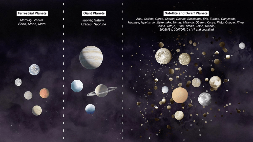
Example: World Map in a one dimensaional view (1D)

1 D Radiative Model (Output)
In a 1 D = one dimensional model the ball (the three dimensional) shape of the earth or any other planet is neglected. A sort of “flat earth” perspecitve is taken and the climate is seen as a number of layers on top of each other towering this flat model structure. Each layer is seen as the average of the climate at that altitude. This simplification is taken to optimize computation.
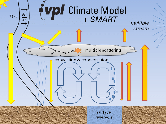
Image Reference
Shows how cloud will reduce the radiation of the planet. Below the clouds convection zones will form.Result: Radiative-convective model (Output) – see page 6 in the paper
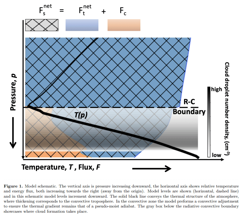

F the flux of radiative energy through each layer with clouds
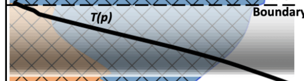
Clouds can form under these conditions and are shown in the diagram by the gray box. The key conditions are certain pressure (range) at a certain temperature (range). And the change in gray colour represents the density of the cloud droplets in the cloud.

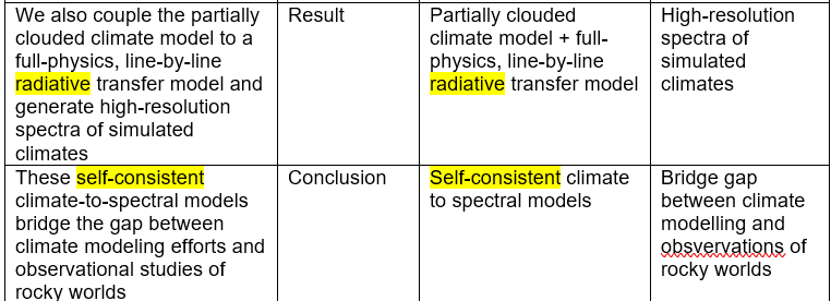
High resolution spectra example (Result Output) :
or AI generated with Stable Diffusion :

Simulated Climate example (Result Output):
This may look like a slow process, yet it is quite the opposite. In order to speed it up is to slow down first, which is rather counter-intuitive. With every new abstract in this topic area, the process will become easier and faster.
Maintaining the flow keeps the momemtum
Aim of the method is to keep the flow even under the worst conditions by breaking it into very small steps (example sentences) and switching between mental demanding (e.g. analysing the sentence) and less demanding tasks (e.g. finding an image). These steps can be performed whenever there is a short window of opportunity for example waiting for the next meeting, waiting for a bus, etc. The idea is to never have to schedule time for reading an abstract or to wait for the ideal moment to come.
Productivity rule: One piece flow versus backlog building
Instead of piling up a backlog of papers in the initial search, work on one paper first until completion of the analysis before looking for the next paper.
Reading an abstract this way is ideal for scoping research and searching for new research questions to address. In this case looking additionally at the discussion section towards the end of the paper and there mainly at the future work section will help identifying the open research questions.
If you do already have a research topic and are working on a literature review, not all detailed steps of such an anlaysis are needed. At any point of the reading you might come to the conclusion that this paper is not helping your research topic and therefore you will turn to the next paper.
Appendix:
The overall table of the abstract.
Sentence Section Input Output Clouds are ubiquitous — they arise for every solar system planet that possesses an atmosphere and have also been suggested as a leading mechanism for obscuring spectral features in exoplanet observations Introduction Solar System Planet with Atmosphere – clouds Observations: Clouds – Obscuring spectral features Observation Exoplanet – spectral features obscured As exoplanet observations continue to improve, there is a need for efficient and general planetary climate models that appropriately handle the possible cloudy atmospheric environments that arise on these worlds Introduction Efficient and general climate modes for cloudy atmospheric environments Improve Exoplanet observation We generate a new 1D radiative-convective terrestrial planet climate model that selfconsistently handles patchy clouds through a parameterized microphysical treatment of condensation and sedimentation processes Method Condensation and sedimatation processes Patchy Clouds Selfconsistently handled through a parametrized microphysical treatment 1D radiative-convective terrestrial planet climate model Our model is general enough to recreate Earth’s atmospheric radiative environment without over-parameterization, while also maintaining a simple implementation that is applicable to a wide range of atmospheric compositions and physical planetary properties Method Model without overparamterization, wide range of atmospheric composition and planetary properties Recreate Earth’s atmospheric radiative environment; implementation for other planets with atmosphere We first validate this new 1D patchy cloud radiative-convective climate model by comparing it to Earth thermal structure data and to existing climate and radiative transfer tools Method Comparison to thermal earth structure data and to existing climate and radiative transfer tools 1D patchy cloud radiative-convective climate model validated We produce partially-clouded Earth-like climates with cloud structures that are representative of deep tropospheric convection and are adequate 1D representations of clouds within rocky planet atmospheres Method Partially.clouded Earth like climates with cloud structures of deep tropospheric convection 1D Earth-like climates with cloud structures for rocky planets with atmosphere After validation against Earth, we then use our partially clouded climate model and explore the potential climates of superEarth exoplanets with secondary nitrogen-dominated atmospheres which we assume are abiotic Method Validated partially clouded climate model Climates of superEarth exoplanets with nitrogen-dominated atmospheres and no life We also couple the partially clouded climate model to a full-physics, line-by-line radiative transfer model and generate high-resolution spectra of simulated climates Result Partially clouded climate model + full-physics, line-by-line radiative transfer model High-resolution spectra of simulated climates These self-consistent climate-to-spectral models bridge the gap between climate modeling efforts and observational studies of rocky worlds Conclusion Self-consistent climate to spectral models Bridge gap between climate modelling and obsvervations of rocky worlds The output and input might be messy in the first pass. With each new pass through it will get clearer.
Further AI assisted Reading
Semantic Scholar | Semantic Reader
AI-Powered Augmented Scientific Reading Application to overcome the following obstacles:
- Frequently paging back and forth looking for the details of cited papers
- Challenges recognizing the same work across multiple papers
- Losing track of reading history and notes
- Contending with a PDF format that is not well suited to mobile reading or assistive technologies such as screen readers
AI assisted Literature Review Process
-
Convection – Research Community
Who is who in the convection research, which scientific journals are publishing these scientific papers, what are the key conferences, what are the key arguments used, etc…..
Method of Research: Arxiv Papers by Google Rank United States (14.06.2023)
Search Term: arxiv.org planet convection
List of papers as data source:
- A Radiative-Convective Model for Terrestrial Planets with Self-Consistent Patchy Clouds
- Atmospheric convection plays a key role in the climate of tidally-locked terrestrial exoplanets: insights from high-resolution simulations
- Layered semi-convection and tides in giant planet interiors
- 3D convection-resolving model of temperate, tidally-locked exoplanets
- Thermal Evolution and magnetic history of rocky planets
- Compositional Convection in the Deep Interior of Uranus
- Convection and Mixing in Giant Planet Evolution
- Continuous reorientation of synchronous terrestrial planets controlled by mantle convection
- Thermal convection in the crust of the dwarf planet (1) Ceres
- Layered semi-convection and tides in giant planet interiors – II. Tidal dissipation
- Work in Progress – more to follow
Name Institution Google Rank James D. Windsor Department of Astronomy and Planetary Science, Northern Arizona University, Habitability, Atmospheres, and Biosignatures Laboratory, University of Arizona, NASA Nexus for Exoplanet System Science Virtual Planetary Laboratory, University of Washington 1 Tyler D. Robinson Lunar & Planetary Laboratory, University of Arizona, Department of Astronomy and Planetary Science, Northern Arizona University, Habitability, Atmospheres, and Biosignatures Laboratory, University of Arizona, NASA Nexus for Exoplanet System Science Virtual Planetary Laboratory, University of Washington 1 Ravi kumar Kopparapu 5NASA Goddard Space Flight Center, Greenbelt 1 David E. Trilling Department of Astronomy and Planetary Science, Northern Arizona University 1 Joe LLama Lowell Observatory, Flagstaff. Arizona 1 Amber Young Department of Astronomy and Planetary Science, Northern Arizona University, Habitability, Atmospheres, and Biosignatures Laboratory, University of Arizona, NASA Nexus for Exoplanet System Science Virtual Planetary Laboratory, University of Washington 1 Denis E. Sergeev Department of mathematics
College of Engineering, Mathematics, and Physical Sciences, University of Exeter2 F. Hugo Lambert Department of mathematics
College of Engineering, Mathematics, and Physical Sciences, University of Exeter2 Nathan J. Mayne Department of astrophysics
College of Engineering, Mathematics, and Physical Sciences, University of Exeter2 Ian A. Boutle Department of astrophysics
College of Engineering, Mathematics, and Physical Sciences, University of Exeter, Met Office, Fitzroy Road, Exeter2 James Manners Met Office, Fitzroy Road, Exeter, Global Systems Institute, University of Exeter 2 Krisztian Kohary Department of astrophysics
College of Engineering, Mathematics, and Physical Sciences, University of Exeter2 Quentin André Laboratoire AIM Paris-Saclay, CEA/DRF – CNRS – Universit´e Paris-Diderot 3 Stéphane Mathis Laboratoire AIM Paris-Saclay, CEA/DRF – CNRS – Universit´e Paris-Diderot, LESIA, Observatoire de Paris, PSL Research University, CNRS, Sorbonne Universits 3 A. J. Barker Department of Applied Mathematics, School of Mathematics, University of Leeds 3 Maxence Lefèvre Department of Physics (Atmospheric, Oceanic and Planetary Physics),
University of Oxford4 Martin Turbet 2Observatoire Astronomique de l’Université de Genève 4 Raymond Pierrehumbert Department of Physics (Atmospheric, Oceanic and Planetary Physics),
University of Oxford4 Jisheng Zhang Department of Astronomy and Astrophysics, the University of Chicago 5 Leslie A. Rogers Department of Astronomy and Astrophysics, the University of Chicago 5 Dustin J. Hill Department of Physics, Drexel University, Philadelphia 6 Krista M. Soderlund Institute for Geophysics, Jackson School of Geosciences, University of Texas at Austin 6 Stephen L. W. McMillan Department of Physics, Drexel University, Philadelphia 6 Allona Vazan Department of Geophysics, Atmospheric, and Planetary Sciences Tel-Aviv University 7 Ravit Helled Department of Geophysics, Atmospheric, and Planetary Sciences Tel-Aviv University 7 Attay Kovetz Department of Geophysics, Atmospheric, and Planetary Sciences Tel-Aviv University 7 Morris Podolak Department of Geophysics, Atmospheric, and Planetary Sciences Tel-Aviv University 7 Jeremy Leconte Laboratoire d’astrophysique de Bordeaux, Univ. Bordeaux 8 Michelangelo Formisano INAF-IAPS, Rome 9 C. Federico INAF-IAPS, Rome 9 J. Castillo-Rogez Jet Propulsion Laboratory, California Institute of Tecnhology, Pasadena, 9 M.C. De Sanctis INAF-IAPS, Rome 9 G. Magni INAF-IAPS, Rome 9 Quentin André Laboratoire AIM Paris-Saclay, CEA/DRF – CNRS – Universit´e Paris-Diderot 10 Stéphane Mathis Laboratoire AIM Paris-Saclay, CEA/DRF – CNRS – Universit´e Paris-Diderot, LESIA, Observatoire de Paris, PSL Research University, CNRS, Sorbonne Universits 10 Adrian J. Barker Department of Applied Mathematics, School of Mathematics, University of Leeds 10 Researcher and Institution
Citations
Number of Citations Google Rank 0 1 46 2 24 3 17 4 1 5 0 6 52 7 0 8 4 9 14 10 Scientific Journal or other Publications
Publication Google Rank 1 ApJ – The Astrophysical Journal 2 SF2A 2017 proceeding 3 ApJ – The Astrophysical Journal 4 ApJ – The Astrophysical Journal 5 6 ApJ – The Astrophysical Journal 7 Nature Geoscience 8 MNRAS 9 Astronomy & Astrophysics 10 Latest Discussion
After analysing the community and understanding their channels is next to have a look at the latest discussion within the community and where the research is heading.
Research Method: Arxiv Papers Google Rank (14.06.2023)
Past Year
- A Radiative-Convective Model for Terrestrial Planets with Self-Consistent Patchy Clouds
- Convection and Clouds under Different Planetary Gravities Simulated by a Small-domain Cloud-resolving Model
- Thermal Evolution and magnetic history of rocky planets
- Convective outgassing efficiency in planetary magma oceans: insights from computational fluid dynamics
- Synergies between Venus & Exoplanetary Observations
Most popular disucssion:
Google Rank overall match with latest Discussion in the last year – papers in both list with Google Rank overall highest define the most popular discussion based on Google Rank.
Author Guidelines Scientific Journals
ApJL – The Astrophysical Journal Letters
